Rapid advances in hardware have been transforming revolutionary approaches in computer graphics into reality. One typical example is the raster graphics that took place in the seventies, when hardware innovations enabled the transition from vector graphics to raster graphics. Another example, which has a similar potential, is currently shaping up in the field of volume graphics. This trend is rooted in the extensive research and development effort in scientific visualization in general and in volume visualization in particular.

Visualization is the usage of computer-supported, interactive, visual representations of data to amplify cognition. Scientific visualization is the visualization of physically based data. Volume visualization is a method of extracting meaningful information from volumetric datasets through the use of interactive graphics and imaging, and is concerned with the representation, manipulation, and rendering of volumetric datasets. Its objective is to provide mechanisms for peering inside volumetric datasets and to enhance the visual understanding.

Traditional 3D graphics is based on surface representation. Most common form is polygon-based surfaces for which affordable special-purpose rendering hardware have been developed in the recent years. Volume graphics has the potential to greatly advance the field of 3D graphics by offering a comprehensive alternative to conventional surface representation methods.

Our display screens are composed of a two-dimensional array of pixels each representing a unit area. A volume is a three-dimensional array of cubic elements, each representing a unit of space. Individual elements of a three-dimensional space are called volume elements or voxels. A number associated with each point in a volume is called the value at that point. The collection of all these values is called a scalar field on the volume. The set of all points in the volume with a given scalar value is called a level surface. Volume rendering is the process of displaying scalar fields. It is a method for visualizing a three-dimensional data set. The interior information about a data set is projected to a display screen using the volume rendering methods. Along the ray path from each screen pixel, interior data values are examined and encoded for display. How the data are encoded for display depends on the application. Seismic data, for example, is often examined to find the maximum and minimum values along each ray. The values can then be color coded to give information about the width of the interval and the minimum value. In medical applications, the data values are opacity factors in the range from 0 to 1 for the tissue and bone layers. Bone layers are completely opaque, while tissue is somewhat transparent. Voxels represent various physical characteristics, such as density, temperature, velocity, and pressure. Other measurements, such as area, and volume, can be extracted from the volume datasets. Applications of volume visualization are medical imaging (e.g., computed tomography, magnetic resonance imaging, ultrasonography), biology (e.g., confocal microscopy), geophysics (e.g., seismic measurements from oil and gas exploration), industry (e.g., finite element models), molecular systems (e.g., electron density maps), meteorology (e.g., stormy (prediction), computational fluid dynamics (e.g., water flow), computational chemistry (e.g., new materials), digital signal and image processing (e.g., CSG ). Numerical simulations and sampling devices such as magnetic resonance imaging (MRI), computed tomography (CT), positron emission tomography (PET), ultrasonic imaging, confocal microscopy, supercomputer simulations, geometric models, laser scanners, depth images estimated by stereo disparity, satellite imaging, and sonar are sources of large 3D datasets.

3D scientific data can be generated in a variety of disciplines by using sampling methods. Volumetric data obtained from biomedical scanners typically come in the form of 2D slices of a regular, Cartesian grid, sometimes varying in one or more major directions. The typical output of supercomputer and Finite Element Method (FEM) simulations is irregular grids. The raw output of an ultrasound scan is a sequence of arbitrarily oriented, fan-shaped slices, which constitute partially structured point samples. A sequence of 2D slices obtained from these scanners is reconstructed into a 3D volume model. Imaging machines have a resolution of millimeters scale so that many details important for scientific purposes can be recorded.

It is often necessary to view the dataset from continuously changing positions to better understand the data being visualized. The real-time interaction is the most essential requirement and preferred even if it is rendered in a somewhat less realistic way. A real-time rendering system is important for the following reasons:

· to visualize rapidly changing datasets,

· for real-time exploration of 3D datasets, (e.g. virtual reality)

· for interactive manipulation of visualization parameters, (e.g. classification)

· for interactive volume graphics.

Rendering and processing does not depend on the object’s complexity or type, it depends only on volume resolution. The dataset resolutions are generally anywhere from 128³ to 1024³ and may be non-symmetric (i.e. 1024 x 1024 x 512).

1.2 Volumetric Data

Volumetric data is typically a set of samples S(x, y, z, v), representing the value v of some property of the data, at a 3D location (x, y, z). If the value is simply a 0 or a 1, with a value of 0 indicating background and a value of 1 indicating the object, then the data is referred to as binary data. The data may instead be multi-valued, with the value representing some measurable property of the data, including, for example, color, density, heat or pressure. The value v may even be a vector, representing, for example, velocity at each location. In general, the samples may be taken at purely random locations in space, but in most cases the set S is isotropic containing samples taken at regularly spaced intervals along three orthogonal axes. When the spacing between samples along each axis is a constant, then S is called isotropic, but there may be three different spacing constants for the three axes. In that case the set S is anisotropic. Since the set of samples is defined on a regular grid, a 3D array (called also volume buffer, cubic frame buffer, 3D raster) is typically used to store the values, with the element location indicating position of the sample on the grid. For this reason, the set S will be referred to as the array of values S(x, y, z), which is defined only at grid locations. Alternatively, either rectilinear, curvilinear (structured), or unstructured grids, are employed (Figure 1‑1).

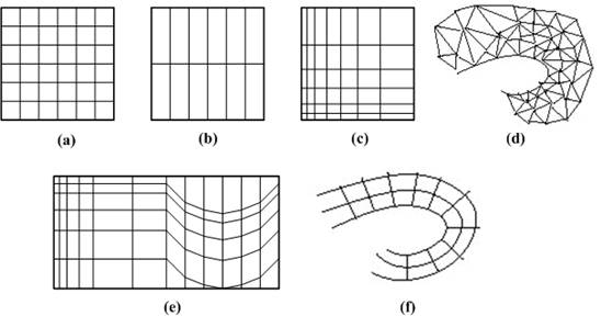
Figure 1‑1: Grid types in volumetric data. a. Cartesian grid, b. Regular grid, c. Rectilinear grid, d. Curvilinear grid, e. Block structured grid, and f. Unstructured grid

In a rectilinear grid the cells are axis-aligned, but grid spacing along the axes are arbitrary. When such a grid has been non-linearly transformed while preserving the grid topology, the grid becomes curvilinear. Usually, the rectilinear grid defining the logical organization is called computational space, and the curvilinear grid is called physical space. Otherwise the grid is called unstructured or irregular. An unstructured or irregular volume data is a collection of cells whose connectivity has to be specified explicitly. These cells can be of an arbitrary shape such as tetrahedra, hexahedra, or prisms.

The array S only defines the value of some measured property of the data at discrete locations in space. A function f(x, y, z) may be defined over the volume in order to describe the value at any continuous location. The function f(x, y, z) = S(x, y, z) if (x, y, z) is a grid location, otherwise f(x, y, z) approximates the sample value at a location (x, y, z) by applying some interpolation function to S. There are many possible interpolation functions. The simplest interpolation function is known as zero-order interpolation, which is actually just a nearest-neighbor function. The value at any location in the volume is simply the value of the closest sample to that location. With this interpolation method there is a region of a constant value around each sample in S. Since the samples in S are regularly spaced, each region is of a uniform size and shape. The region of the constant value that surrounds each sample is known as a voxel with each voxel being a rectangular cuboid having six faces, twelve edges, and eight corners.

Higher-order interpolation functions can also be used to define f(x, y, z) between sample points. One common interpolation function is a piecewise function known as first-order interpolation, or trilinear interpolation. With this interpolation function, the value is assumed to vary linearly along directions parallel to one of the major axes.

1.3 Voxels and cells

Volumes of data are usually treated as either an array of voxels or an array of cells. These two approaches stem from the need to resample the volume between grid points during the rendering process. Resampling, requiring interpolation, occurs in almost every volume visualization algorithm. Since the underlying function is not usually known, and it is not known whether the function was sampled above the Nyquist frequency, it is impossible to check the reliability of the interpolation used to find data values between discrete grid points. It must be assumed that common interpolation techniques are valid for an image to be considered valid.

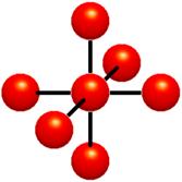
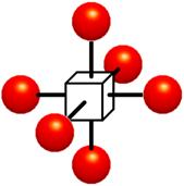
Figure 1‑2: Voxels. Each grid point has a sample value. Data values do not vary within voxels.

The voxel approach dictates that the area around a grid point has the same value as the grid point (Figure 1‑2). A voxel is, therefore, an area of non-varying value surrounding a central grid point. The voxel approach has the advantage that no assumptions are made about the behavior of data between grid points; only known data values are used for generating an image.

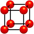
Figure 1‑3 : Cells. Data values do vary within cells. It is assumed that values between grid points can be estimated. Interpolation is used

The cell approach views a volume as a collection of hexahedra whose corners are grid points and whose value varies between the grid points (Figure 1‑3). This technique attempts to estimate values inside the cell by interpolating between the values at the corners of the cell. Trilinear and tricubic are the most commonly used interpolation functions. Images generated using the cell approach, appear smoother than those images created with the voxel approach. However, the validity of the cell-based images cannot be verified.

1.4 Problems Associated with Volume Rendering

As mentioned before, volume visualization is the technique of displaying two-dimensional projections of three-dimensional (volume) data. Data may be acquired from various scanners, such as an MRI, CT, SPECT, or US scanner. Visualizing a given three dimensional dataset can be done using two different approaches based on the portion of the volume raster set which they render; surface rendering, and volume rendering. Surface rendering algorithms first fit geometric primitives to values in the data, and then render these primitives. Since surface rendering algorithms require an intermediate representation, they are less attractive. Volume rendering algorithms render voxels in the volume raster directly, without converting to geometric primitives or first converting to a different domain and then rendering from that domain. They usually include an illumination model, which supports semi-transparent voxels.

Volume rendering can produce informative images that can be useful in data analysis, but a major drawback of the techniques is the time required to generate a high-quality image. An interactive volume visualization scheme requires a performance in the order of Terra (10¹²) operations per second. General-purpose processors alone cannot provide such a performance, and so, additional solutions must be explored. Several volume rendering optimizations have been developed which decrease rendering times, and therefore increase interactivity and productivity. For the optimization of volume visualization there are five main approaches: data reduction by means of model extraction or data simplification, software-based algorithm optimization and acceleration, implementation on general purpose parallel architectures, use of contemporary off-the-shelf graphics hardware, and realization of special-purpose volume rendering engines.

Software based optimizations are divided into two broad groups according to the rendering methods they use, that is, optimization methods for object-space rendering, and image-space rendering. The image-space optimization methods are based on the observation that most of the existing methods for speeding up the process of ray casting rely on one or more of the following principles: pixel-space coherency, object-space coherency, inter-ray coherency, frame coherency, space-leaping, vertical coherency, temporal coherency, and stereoscopic coherency.

The most effective branch of volume rendering acceleration techniques involve the utilization of the fifth principle: speeding up ray casting by providing efficient means to traverse the empty space, that is space leaping . The passage of a ray through the volume is two phased. In the first phase, the ray advances through the empty space searching for an object. In the second phase, the ray integrates colors and opacities as it penetrates the object. Since the passage of empty space does not contribute to the final image, skipping the empty space provides a significant speed up without affecting the image quality.

The optimization techniques will be examined in more detail in the next chapter.

2 Optimization in VR

2.1 Basics of Optimization

Volume rendering can produce informative images that can be useful in data analysis, but a major drawback of the techniques is the time required to generate a high-quality image. Several volume rendering optimizations are developed which decrease rendering times, and therefore increase interactivity and productivity It is obvious that one can not hope to have a real time volume rending in the near future without investing time, effort, and ingenuity in accelerating the process through software optimizations and hardware implementations. There are five main approaches to overcoming this seemingly insurmountable performance barrier:

1. Data reduction by means of model extraction or data simplification,

2. Software-based algorithm optimization and acceleration,

3. Implementation on general-purpose parallel architectures,

4. Use of contemporary off-the-shelf graphics hardware, and

5. Realization of special-purpose volume rendering engines.

2.2 Task and data decomposition

Since the work is essentially defined as “operations on data”, the choice of task decomposition has a direct impact on data access patterns. On distributed memory architectures, where remote memory references are usually much more expensive than local memory references, the issues of task decomposition and data distribution are inseparable. Shared memory systems offer more flexibility, since all processors have an equal access to the data. While data locality is still important in achieving good caching performance, the penalties for global memory references tend to be less severe, and static assignment of data to processors is not generally required.

There are two main strategies for task decomposition. In an object-parallel approach, tasks are formed by partitioning either the geometric description of the scene or the associated object space. Rendering operations are then applied in parallel to subsets of the geometric data, producing pixel values which must then be integrated into a final image. In contrast, image-parallel algorithms reverse this mapping. Tasks are formed by partitioning the image space, and each task renders the geometric primitives which contribute to the pixels which it has been assigned. To achieve a better balance among the various overheads, some algorithms adopt a hybrid approach, incorporating features of both object- and image-parallel methods. These techniques partition both the object and image spaces, breaking the rendering pipeline in the middle and communicating intermediate results from object rendering tasks to image rendering tasks.

Volume rendering algorithms typically loops through the data, calculating the contribution of each volume sample to pixels on the image plane. This is a costly operation for moderate to large sized data, leading to rendering times that are non-interactive. Viewing the intermediate results in the image plane may be useful, but these partial image results are not always representatives of the final image. For the purpose of interaction, it is useful to be able to generate a lower quality image in a shorter amount of time, which is known as data simplification. For data sets with binary sample values, bits could be packed into bytes such that each byte represents a 2´2´2 portion of the data. The data would be processed bit-by-bit to generate the full resolution image, but lower resolution image could be generated by processing the data byte-by-byte. If more than four bits of the byte are set, the byte is considered to represent an element of the object, otherwise it represents the background. This will produce an image with one-half the linear resolution in approximately one eighth the time.

2.3 Software-based algorithm optimization and acceleration

Software based algorithm optimizations are divided into two broad groups according to the rendering methods they use, that is optimization methods for object-space rendering and image-space rendering. The methods that have been suggested to reduce the amount of computations needed for the transformation by exploiting the spatial coherency between voxels for object-space rendering are:

1. Recursive “divide and conquer”,

2. pre-calculated tables,

3. incremental transformation, and

4. shearing-based transforms.

The major algorithmic strategy for parallelizing volume rendering is the divide-and-conquer paradigm. The volume rendering problem can be subdivided either in data space or in image space. Data-space subdivision assigns the computation associated with particular sub volumes to processors, while image-space subdivision distributes the computation associated with particular portions of the image space. This method exploits coherency in voxel space by representing the 3D volume by an octree. A group of neighboring voxels having the same value may, under some restrictions, be grouped into a uniform cubic sub volume. This aggregate of voxels can be transformed and rendered as a uniform unit instead of processing each of its voxels.

The table-driven transformation method is based on the observation that volume transformation involves the multiplication of the matrix elements with integer values which are always in the range of volume resolution. Therefore, in a short preprocessing stage each matrix element is allocated a table. All the multiplication calculations required for the transformation matrix multiplication are stored into a look-up table. The transformation of a voxel can then be accomplished simply by accessing the look-up table, the entry accessed in the table depending on the xyz coordinates of the voxel. During the transformation stage, coordinate by matrix multiplication is replaced by table lookup.

The incremental transformation method is based on the observation that the transformation of a voxel can be incrementally computed given the transformed vector of the voxel. To employ this approach, all volume elements, including the empty ones, have to be transformed. This approach is especially attractive for vector processors since the transformations of the set of voxels can be computed from the transformation of the vector by adding, to each element in this vector. Another method exploits coherency within the volume to implement a novel incremental transformation scheme. A seed voxel is first transformed using the normal matrix-vector multiplication. All other voxels are then transformed in an incremental manner with just three extra additions per coordinate.

The shearing algorithm decomposes the 3D affine transformation into five 1D shearing transformations. The major advantage of this approach is its ability (using simple averaging techniques) to overcome some of the sampling problems causing the production of low quality images. In addition, this approach replaces the 3D transformation by five 1D transformations which require only one floating-point addition each.

The image-space optimization methods are based on the observation that most of the existing methods for speeding up the process of ray casting rely on one or more of the following principles:

1. Pixel-space coherency,

2. object-space coherency,

3. inter-ray coherency,

4. frame coherency, and

5. space-leaping.

Pixel-space coherency means that there is a high coherency between pixels in the image space. It is highly probable that between two pixels having identical or similar color we will find another pixel having the same or similar color. Therefore, it might be the case that we could avoid sending a ray for such obviously identical pixels.

Object-space coherency means that there is coherency between voxels in the object space. Therefore, it should be possible to avoid sampling in 3D regions having uniform or similar values. In this method the ray starts sampling the volume in a low frequency (i.e., large steps between sample points). If a large value difference is encountered between two adjacent samples, additional samples are taken between them to resolve ambiguities in these high frequency regions.

Inter-ray coherency means that, in parallel viewing, all rays have the same form and there is no need to reactivate the discrete line algorithm for each ray. Instead, we can compute the form of the ray once and store it in a data structure called the ray-template. Since all the rays are parallel, one ray can be discretized and used as a ‘‘template’’ for all other rays.

Frame coherency means that when an animation sequence is generated, in many cases, there is not much difference between successive images. Therefore, much of the work invested to produce one image may be used to expedite the generation of the next image.

The most prolific and effective branch of volume rendering acceleration techniques involve the utilization of the fifth principle: speeding up ray casting by providing efficient means to traverse the empty space, that is space leaping. The passage of a ray through the volume is two phased. In the first phase the ray advances through the empty space searching for an object. In the second phase the ray integrates colors and opacities as it penetrates the object. Since the passage of empty space does not contribute to the final image it is observed that skipping the empty space could provide a significant speed up without affecting the image quality.

2.4 Parallel and distributed architectures

The need for interactive or real-time response in many applications places additional demands on processing power. The only practical way to obtain the needed computational power is to exploit multiple processing units to speed up the rendering task, a concept which has become known as parallel rendering.

Several different types of parallelism can be applied in the rendering process. These include functional parallelism, data parallelism, and temporal parallelism. Some are more appropriate to specific applications or specific rendering methods, while others have a broader applicability. The basic types can also be combined into hybrid systems which exploit multiple forms of parallelism.

One way to obtain parallelism is to split the rendering process into several distinct functions which can be applied in series to individual data items. If a processing unit is assigned to each function (or group of functions) and a data path is provided from one unit to the next, a rendering pipeline is formed. As a processing unit completes work on one data item, it forwards it to the next unit, and receives a new item from its upstream neighbor. Once the pipeline is filled, the degree of parallelism achieved is proportional to the number of functional units. The functional approach works especially well for polygon and surface rendering applications.

Instead of performing a sequence of rendering functions on a single data stream, it may be preferable to split the data into multiple streams and operate on several items simultaneously by replicating a number of identical rendering units. The parallelism achievable with this approach is not limited by the number of stages in the rendering pipeline, but rather by economic and technical constraints on the number of processing units which can be incorporated into a single system.

In animation applications, where hundreds or thousands of high-quality images must be produced for a subsequent playback, the time to render individual frames may not be as important as the overall time required to render all of them. In this case, parallelism may be obtained by decomposing the problem in the time domain. The fundamental unit of work is a complete image, and each processor is assigned a number of frames to render, along with the data needed to produce those frames.

It is certainly possible to incorporate multiple forms of parallelism in a single system. For example, the functional- and data-parallel approaches may be combined by replicating all or a part of the rendering pipeline

2.5 Commercial graphics hardware

One of the most common resources for rendering is off-the-shelf graphics hardware. However, these polygon rendering engines seem inherently unsuitable to the task. Recently, some new methods have tapped to this rendering power by either utilizing texture mapping capabilities for rendering splats, or by exploiting solid texturing capabilities to implement a slicing-based volume rendering. The commercially available solid texturing hardware allows mapping of volumes on polygons using these methods. These 3D texture maps are mapped on polygons in 3D space using either zero order or first order interpolation. By rendering polygons, slicing the volume and perpendicular to the view direction one generates a view of a rectangular volume data set.

2.6 Special purpose hardware

To fulfill the special requirements of high-speed volume visualization, several architectures have been proposed and a few have been built. The earliest proposed volume visualization system was the “Physician’s Workstation” which proposed real-time medical volume viewing using a custom hardware accelerator. The Voxel Display Processor (VDP) was a set of parallel processing elements. A 64³ prototype was constructed which generated 16 arbitrary projections each second by implementing depth-only-shading. Another system which presented a scalable method was SCOPE architecture. It was also implementing the depth-only-shading scheme.

The VOGUE architecture was developed at the University of Tübingen, Germany. A compact volume rendering accelerator, which implements the conventional volume rendering ray casting pipeline proposed in [1], originally called the Voxel Engine for Real-time Visualization and Examination (VERVE), achieved 2.5 frames/second for 256³datasets.

The design of VERVE [2] was reconsidered in the context of a low cost PCI coprocessor board. This FPGA implementation called VIZARD was able to render 10 perspective, ray cast, and grayscale 256 x 200 images of a 256² x 222 volume per second.

VIZARD II architecture is at the University of Tübingen to bring interactive ray casting into the realm of desktop computers and was designed to interface to a standard PC system using the PCI bus. It sustained a frame rate of 10 frames/second in a 256³ volume (Figure 2‑1).

Figure 2‑1: VIZARD II co-processor card

In DOGGETT system an array-based architecture for volume rendering is described. It performs ray casting by rotating planes of voxels with a warp array, then passing rays through it in the ray array. The estimated performance for an FPGA implementation is 15 frames/second yielding 384² images of 256³ data sets.

The VIRIM architecture [3] has been developed and assembled in the University of Mannheim which implements the Heidelberg ray tracing model, to achieve real-time visualization on moderate sized (256 x 256 x 128) datasets with a high image quality. VIRIM was capable of producing shadows and supports perspective projections. One VIRIM module with four boards has been assembled and achieved 2.5 Hz frame rates for 256 x 256 x 128 datasets. To achieve interactive frame rates, multiple rendering modules have to be used; however, dataset duplication was required. Four modules (16 boards) were estimated to achieve 10 Hz for the same dataset size, and eight modules (32 boards) were estimated to achieve 10 Hz for 256³ datasets.

VIRIM II [4] improved on VIRIM by reducing the memory bottleneck. The basic design of a single memory interface was unchanged. To achieve higher frame rates or to handle higher resolutions, multiple nodes must be connected on a ring network that scales with the number of nodes. It was predicted that using 512 nodes, a system could render 2048³ datasets at 30 Hz..

The hierarchical, object order volume rendering architecture BELA, with eight projection processors and image assemblers, was capable of rendering a 256³ volume into an image at a 12 Hz rendering rate [5].

The Distributed Volume Visualization Architecture [6], DIV²A, was an architecture that performed conventional ray casting with a linear array of custom processors. To achieve 20Hz frame rates with a 256³ volume, 16 processing elements using several chips each were required.

The volume rendering architecture with the longest history is the Cube family. Beginning with Cube-1 and spanning to Cube-4 and beyond, the architecture provides a complete, real-time volume rendering visualization system. A mass market version of Cube-4 was introduced in 1998 providing real-time volume rendering of 256³ volumes at 30 Hz for inclusion in a desktop personal computer [6].

The Cube-1 concept was proven with a wire-wrapped prototype (Figure 2‑2). 2D projections were generated at a frame rate of 16 Hz for a 512³ volume. The main problems with the implementation of Cube-1 were the large physical size and the long settling time. To improve these characteristics, Cube-2 was developed [6].

Figure 2‑2: A 16³ resolution prototype of Cube-1 architecture

Cube-2 [7] implemented a 16³ VLSI version of Cube-1 (Figure 2‑3). A single chip contained all the memory and processing of a whole Cube-1 board.

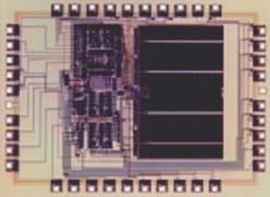
Figure 2‑3: A 16³ resolution Cube-2 VLSI implementation

Although the prior Cube designs were fast, the foundations of volume sampling and rendering were not fully developed so the architecture was unable to provide higher order sampling and shading. Cube-3 [8] improved the quality of rendering by supporting full 3D interpolation of samples along a ray, accurate gray-level gradient estimation, and flexible volumetric shading and provided real-time rendering of 512³ volumes.

Due to the capability of providing real-time rendering, the cost and size of the Cube-3 was unreasonable. This prompted the development of Cube-4 [9] which avoided all global communication, except at the pixel level and achieved rendering in 128³ datasets in 0.65 seconds at 0.96 MHz processing frequency. There is also a new version Cube-4L which is currently being implemented by Japan Radio Co. as part of a real-time 3D ultrasound scanner [6, 10].

EM-Cube is a commercial version of the high-performance Cube-4 volume rendering architecture that was originally developed at the State University of New York at Stony Brook, and is implemented as a PCI card for Windows NT computers. EM-Cube is a parallel projection engine with multiple rendering pipelines. Eight pipelines operating in parallel can process 8 x 66 x 10⁶ or approximately 533 million samples per second. This is sufficient to render 256³ volumes at 30 frames per second [6]. It does not support perspective projections.

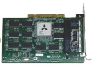
Figure 2‑4: The VolumePro PCI card

VolumePro [11], the first single chip rendering system is developed at SUNY Stony Brook and is based on the Cube-4 volume rendering architecture. VolumePro is the commercial implementation of EM-Cube, and it makes several important enhancements to its architecture and design. VolumePro is now available on a low cost PCI board delivering the best price/performance ratio of any available volume rendering system (Figure 2‑4).

Volume rendering techniques allows us to fully reveal the internal structure of 3D data, including amorphous and semi-transparent features. It encompasses an array of techniques for displaying images directly from 3D data; thus, it has become a key technology in the visualization of scientific volumetric data. Yet, when real time visualization is considered, it is obvious that, without the assistance of a specific hardware, this task cannot be achieved. In the following chapters, a solution to this problem will be examined which makes use of Digital Signal Processors.

3 Framework

3.1 Introduction

This chapter gives the basics of the volume-rendering algorithm which will be the subject of the hardware implementation. It is basically a template-based, discrete ray tracing algorithm. Discrete ray tracing is well known and common in use as it prefers discrete representations of models rather than geometric forms, which therefore provides a substantial improvement in computational speed. “Template” refers to the ray to be traced for every pixel on the image plane into the volume to find the contribution of the data for that pixel. It is an important optimization method for volume rendering. Rays skips empty voxel space, providing a significant speed-up without affecting the image quality, which is also an important optimization of the algorithm and known as space leaping.

3.2 The Pipeline

The rendering pipeline of the visualization algorithm is shown in Figure 3‑1. The organization scheme of the memory module affects the performance of rendering algorithms. The volumetric dataset to be rendered is provided in a standard memory module. It is possible to say that the algorithm suffers from the limited memory performance capabilities of personal computers. To decrease this burden, an 8-bit data structure per voxel is used in the majority of the datasets. Still it is obvious that the speed of a ray-caster depends on the total number of voxels it traverses. Thus, the total rendering time of a volume is a matter of volume resolution, independent of the object complexity within the volume.

Slice extraction is the cheapest part of the pipeline, as it requires nothing but just accessing the correct addresses of the volume data to generate an image. Slice images can be generated in arbitrary angles with each of the spatial axes. Examples are shown in Figure 3‑2.

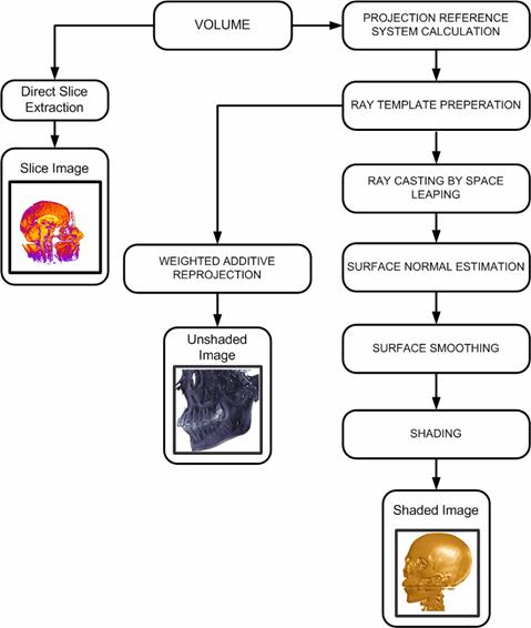
Figure 3‑1: The pipeline of the algorithm

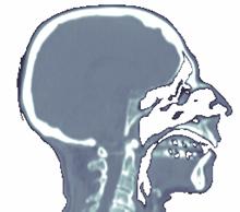
(a) (b)

Figure 3‑2: Slices extracted from the CT dataset. a. Sagittal view, b. axial view

The projection reference system is standard for all graphics applications. The planar geometric projection used by the algorithm is orthogonal projection as it simplifies the algorithm by giving rise to the inter-ray coherency. But spatial address transformation, surface normal estimation, space leaping, and surface smoothing algorithms that are going to be introduced later are applicable for perspective projection as well.

Since parallel projection is used, the direction of projection and the normal to the projection plane are the same in direction. Therefore, all rays have the same form. A discrete line algorithm is activated once per projection, and its elements are recorded in a data structure called ray template, which is essentially a line with 26-connectivity. The usage of the template provides a considerable time/performance benefit to the system. However, this strategy causes the skipping of some voxels for 26-rays, while some others are being visited twice. This phenomenon leads to the employment of a plane other than the view plane, parallel to one of the principle axes, and tracing templates from that plane. It is called base-plane. It was determined which of the volume faces projected to the largest area on the screen-plane that the plane containing this face as the base-plane. The volume is projected onto the base-plane and then perform a 2D image transformation to yield the desired result. The base-plane used in this work is oriented as near as possible to the actual view plane while preserving its parallelism to one of the spatial axes. This leads to the minimization of projection errors originated from the base-plane usage, and therefore eliminates the need for a 2D transformation.

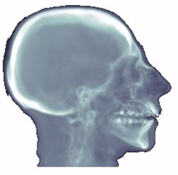
(a) (b)

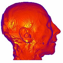
Figure 3‑3: Images generated by two different tracing schemes. a. First-hit projection method, b. weighted additive reprojection method

Commonly, the outcome of the viewing process consists of, for each screen pixel, the depth and the value (color) of the first opaque voxel encountered by the ray emitted from that pixel. This scheme is called first-hit projection. However, it is possible to apply different operators while following the ray. The weighted additive reprojection produces an X-ray-like image by averaging the intensities along the ray. Alternatively, one could display the maximum value encountered along the ray passage, like in a method called maximum projection, or the minimum value encountered called minimum intensity projection. Assigning opacities to voxel values will enable a compositing projection to simulate semitransparent volumes. Two samples are shown in Figure 3‑3. The left image is a first-hit projection without shading and the image on the right is produced by the weighted additive reprojection method. The first opaque voxels found during tracing are provided as input for the shading process

The traversal of volume data consists of two phases, the traversal of the empty space, and the traversal of the occupied voxels. It is obvious that the empty space does not have to be sampled – it has only to be crossed as fast as possible. For all the ray traversal schemes that are included into this pipeline, the empty space is leaped forward. There are many methods that apply to space leaping in the literature. Existing methods require a preprocessing stage, and some require specific rendering methods. Here, a method that independent of the rendering algorithm is used.

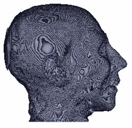
Most ray tracing schemes require a shading model to be used to enhance the understanding of the data. For each voxel, a normal vector is required for the shading stage. As the data in the volume is represented in discrete space, no geometric information is available explicitly, which yields a lack of information. Therefore, a normal vector to the surface of each voxel has to be estimated. This process is called surface-normal estimation. The usage of gradient vector instead of the surface normal is the trend in volume rendering literature.

(a) (b)

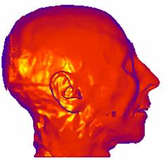
Figure 3‑4: Shaded image of CT dataset. a. Without surface-smoothing, b. with surface smoothing

The method used for the normal estimation, is based on a simple geometric model of the voxel neighborhood. Five polygons are produced from the four neighbors of each voxel and the normal is estimated by averaging these polygon normals. The discrete representation of the data causes an incorrect, patch-like shaded image with the surface normals estimated, as shown in Figure 3‑4.a, and the process of repairing these patches is called surface smoothing. There are several methods in the literature. The method introduced in this work is based on averaging the surface normals exceeding a threshold within a pre-defined kernel. An image with surface smoothing is shown in Figure 3‑4.b. The Phong shading is preferred as the shading model.

3.3 Specification of an Arbitrary 3D View

In general, projections transform points in a coordinate system of dimension n into points in a coordinate system of dimension less than n. In fact, computer graphics has long been used for studying n-dimensional objects by projecting them into 2D for viewing. The projection of a 3D object is defined by straight projection rays, emanating from a center of projection, passing through each point of the object, and intersecting a projection plane to form the projection. The class of projections with which we deal with is known as planar geometric projections. Planar geometric projections can be divided into two basic classes: perspective and parallel. The distinction lies in the relation of the center of projection to the projection plane. If the distance from the one to the other is finite, then the projection is perspective, and if infinite the projection is parallel. When we define a perspective projection, we explicitly specify its center of projection; for a parallel projection, we give its direction of projection. The visual effect of a perspective projection is similar to that of photographic systems and of the human visual system, and is known as perspective foreshortening. The size of the perspective shortening of an object varies inversely with the distance of that object from the center of projection. Thus, although the perspective projection of objects tends to look realistic, it is not particularly useful for recording the exact shape and measurements of the objects; distances cannot be taken from the projection, angles are preserved on only those faces of the object parallel to the projection plane, and parallel lines do not in general project as parallel lines. The parallel projection is a less realistic view because perspective foreshortening is lacking, although there can be different constant foreshortenings along each axis. The projection can be used for exact measurements, and parallel lines do remain parallel. As in the perspective projection, angles are preserved only on faces of the object parallel to the projection plane.

In order to specify an orthographic projection system:

· A reference point on the plane is defined (view reference point VRP )(Figure 3‑5),

· a normal to the plane is defined ( view plane normal VPN ) (Figure 3‑5),

· an up vector is defined (view-up vector VUP) (Figure 3‑6),

· using VRP and VPN, the view plane is calculated,

· the v-axis of the plane is calculated,

· the u-axis of the plane is calculated, (Figure 3‑7) and,

· a window on the plane is defined whose contents are mapped to the viewport for visualization.(Figure 3‑8)

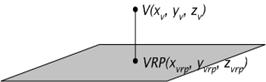
Figure 3‑5: View reference point (VRP) and point V on the view plane

Figure 3‑6: Definition of the view-up vector

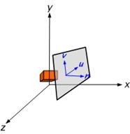
Figure 3‑7: The components of an orthographic projection system

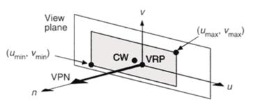
Figure 3‑8: The definition of the window on the view plane

3.4 Ray Template

Voxelization algorithms that convert a 3D continuous line representation into a discrete line representation have two common usages in volume graphics:

1. As the 3D line is a fundamental primitive, it is used as a building block for generating more complex objects. For example, a voxelized cylinder can be generated by sweeping a 3D voxelized circle.

2. It is used for ray traversal in the voxel space. Rendering techniques that cast rays through a volume of voxels are based on algorithms that generate the set of voxels visited by the continuous ray. Discrete ray algorithms have been developed for the traversal of a 3D space partition.

A formal definition of a 3D discrete line is mandatory in numerous applications. The existing methods may be sorted in two categories as:

1. “By projections” method, where two projections of the 3D segment are independently computed on two basic planes, (Figure 3‑9),

2. “By direct calculus” method obtained by an extension of the 2D and 3D algorithms.

A line voxelization algorithm generates a 3D discrete line from a 3D continuous line, which is a set of connected voxels approximating the continuous line.

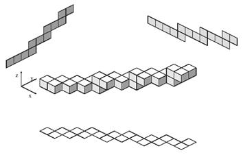
Figure 3‑9: By projections generation method of a 3D discrete line

3.5 Shading

As a result of first-hit projection the data seized by the traced rays are projected onto the view plane. But it is obvious from Figure 3‑4.a that, the image is unpleasant and it cannot support perception. Realistic displays of data can amplify cognition and they can be obtained by applying natural lighting effects to the visible surfaces. An illumination model is used to calculate the intensity of light that should be seen at a given point on the surface of the object. The model developed by Bui-Tuong Phong is preferred as it yields substantial improvements over other models and known as Phong illumination model.

Modeling the colors and lighting effects that is seen on an object is a complex process, involving principles of physics and psychology. Fundamentally, lighting effects are described with a model that considers the interaction of electromagnetic energy with object surfaces. Once light reaches the observer’s eyes, it triggers perception processes that determine what is actually seen in a scene. Phong illumination model involves a number of factors, such as object type, object position relative to light source and other objects, and the light source conditions that are defined for the scene. Objects can be constructed from opaque materials, or they can be more or less transparent. In addition, they can have shiny or dull surfaces, and they can have a variety of surface-texture patterns. Light sources, of varying shapes, colors, and positions, can be used to provide the illumination effects for an image. Given the parameters for the optical properties of surfaces, the relative positions of the surfaces in a scene, the color and positions of the light sources, and the position and orientation of the viewing plane, Phong model calculates the intensity projected from a particular surface point in a specified viewing direction.

Figure 3‑10 and Figure 3‑11 shows the effect of different parameters of shading algorithm, and Figure 3‑12 shows the combined result of shading parameters.

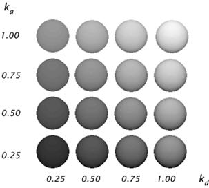
Figure 3‑10: Diffuse reflections from a spherical surface illuminated with ambient light and a single point light source for values of k_a and k_d in the interval (0, 1).

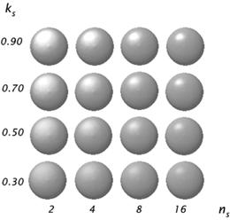
Figure 3‑11: Specular reflections from a spherical surface for varying specular parameter values and a single light source.

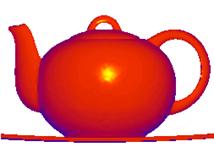
Figure 3‑12: A color model shaded using Phong shading. Diffuse and specular reflections are combined to obtain a complete shading model.

In this chapter, the general structure of the subject of this hardware implementation is presented in a pipelined manner. This pipeline combines several algorithms to extract meaningful information from the given data. The reference of the projection system is almost standard for all graphics applications. Address space transformation is the major subject of this reference system.

The first-hit projection scheme employs ray tracing, which involves an illumination model. A 3D line generator calculates the common form of the rays to be traced. Phong model is used for shading as it provides substantial improvements over the other existing methods. The implementation of a global illumination algorithm invites the normal vectors at each sampling point in the final image. Since there are no such explicit information available with discrete representation scheme of the data, these vectors has to be approximated. This is done with a surface normal estimation algorithm. As a drawback, the final image suffers from some undesired effects, which have to be repaired. The existence of a surface-smoothing algorithm in the pipeline stem from this need. It discards these artifacts and produces pleasing images.

In this chapter, we have also reviewed the methods used in the specification of an arbitrary view, the 3D line generation and the construction of the ray template, and the shading algorithms in detail.

4 Choosing the Right DSP Processor

4.1 Digital Signal Processing

Digital signal processing is a method of processing real world signals (represented by a sequence of numbers) using mathematical techniques to perform transformations or extract information.

We don't speak in a digital signal. A digital signal is a language of 1s and 0s that can be processed by mathematics. We speak in real-world, analog signals. Analog signals are real world signals that we experience everyday - sound, light, temperature, and pressure. A digital signal is a numerical representation of the analog signal. It may be easier and more cost effective to process these signals in the digital world. In the real world, we can convert these signals into digital signals through our analog-to-digital conversion process, process the signals, and if needed, bring the signals back out to the analog world through the digital-to-analog converter (Figure 4‑1).

Figure 4‑1: Digital signal processing logic.

The result is crystal clear sound, with no annoying echoes. That's a basic explanation of what a DSP does. It takes a digital signal and processes it to improve the signal. The improvement may be clearer sound, sharper images, or faster data. And that ability to improve signals is making new breakthroughs such as Internet music and broadband to the home possible.

These real-time processors make up the fastest-growing segment of the semiconductor market and are particularly well suited to handle the demands of processing information, whether as the engine of communications applications, by providing the processing platform for the convergence of the internet and wireless applications, or by enabling breakthroughs in medical imaging or performance audio.

4.2 Choosing the Technology

If a universal microprocessor solution existed with which every design could be realized, the electronics industry wouldn't be a very competitive place. However, typically in most electronic designs, more than one processor technology can be used to implement the required functions. The trick is, of course, to choose the one that best delivers the performance, size, power consumption, features, software and tools to get the job done fast - without breaking the budget. After almost two decades of development, digital signal processors continue to take the place of competitive processors. Digital signal processors are, after all, at the center of signal processing.

4.2.1 Digital Signal Processors (DSP)

A digital signal processor (DSP) is a type of microprocessor - one that is incredibly fast and powerful. A DSP is unique because it processes data in real time. This real-time capability makes a DSP perfect for applications that cannot tolerate any delays. For example, did you ever talk on a cell phone where two people couldn't talk at once? You had to wait until the other person finished talking. If you both spoke simultaneously, the signal was cut--you didn't hear the other person. With today's digital cell phones, which use DSP, we can talk normally. The DSP processors inside cell phones process sounds so rapidly we hear them as quickly as we can speak - in real time.

Here are just some of the advantages of designing with DSPs over other microprocessors:

· Single-cycle multiply-accumulate operations

· Real-time performance, simulation and emulation

· Flexibility

· Reliability

· Increased system performance

· Reduced system cost

4.2.2 Field Programmable Gate Arrays (FPGA)

Field-Programmable Gate Arrays have the capability of being reconfigurable within a system, which can be a big advantage in applications that need multiple trial versions within development. They also offer greater raw performance per specific operation because of the resulting dedicated logic circuit. However, FPGAs are significantly more expensive and typically have much higher power dissipation than DSPs with similar functionality. As such, even when FPGAs are the chosen performance technology in designs such as wireless infrastructure, DSPs are typically used in conjunction with FPGAs to provide greater flexibility, better price/performance ratios, and lower system power.

4.2.3 Application Specific IC (ASIC)

Application-specific ICs can be tailored to perform specific functions extremely well, and can be made quite power efficient. However, since ASICS are not field-programmable, their functionality cannot be iteratively changed or updated while in product development. As such, every new version of the product requires a redesign and trips through the foundry, an expensive proposition, and an impediment. Programmable DSPs, on the other hand, can be updated without changing the silicon, merely change the software program, greatly reducing development costs, and availing aftermarket feature enhancements with mere code downloads. Consequently, more often than not, when we see ASICs in real time signal processing applications, they are typically employed as bus interfaces, glue logic, and/or functional accelerators for a programmable DSP-based system.

4.2.4 General Purpose Procesoors (GPP)

In contrast to ASICs that are optimized for specific functions, general-purpose microprocessors (GPPs) are best suited for performing a broad array of tasks. However, for applications in which the end product must process answers in real time, or must do so while powered by consumer batteries, GPPs comparatively poor real time performance and high power consumption all but rules them out. More and more, these processors are being seen as the dinosaurs of the industry, too encumbered with PC compatibility and desktop features to adapt to the changing real time market place. As the world embraces tiny hand-held wireless-enabled products that require power dissipation measured in milliwatts-not the watts that these processors consume - DSPs are the programmable technology of choice. That trend is bound to continue as digital Internet appliances get smaller, faster and more portable.

4.3 Choosing the Processor

The right DSP processor for a job depends heavily on the application. One processor may perform well for some applications, but be a poor choice for others. With this in mind, one can consider a number of features that vary from one DSP to another in selecting a processor. These features are discussed below.

4.3.1 Arithmetic Format

One of the most fundamental characteristics of a programmable digital signal processor is the type of native arithmetic used in the processor. Most DSPs use fixed point arithmetic, while other processors using floating-point arithmetic. Floating-point arithmetic is a more flexible and general mechanism than fixed-point. With floating-point, system designers have access to wider dynamic range (the ratio between the largest and smallest numbers that can be represented). As a result, floating-point DSP processors are generally easier to program than their fixed point cousins, but usually are also more expensive and have higher power consumption. The increased cost and power consumption result from the more complex circuitry required within the floating-point processor, which implies a larger silicon die. The ease-of-use advantage of floating-point processors is due to the fact that in many cases the programmer doesn’t have to be concerned about dynamic range and precision. In contrast, on a fixed-point processor, programmers often must carefully scale signals at various stages of their programs to ensure adequate numeric precision with the limited dynamic range of the fixed-point processor. Most high-volume, embedded applications use fixed point processors because the priority is on low cost and, often, low power. Programmers and algorithm designers determine the dynamic range and precision needs of their application, either analytically or through simulation, and then add scaling operations into the code if necessary.

For applications that have extremely demanding dynamic range and precision requirements, or where ease of development is more important than unit cost, floating-point processors have the advantage. It’s possible to perform general-purpose floating point arithmetic on a fixed-point processor by using software routines that emulate the behavior of a floating point device. However, such software routines are usually very expensive in terms of processor cycles. Consequently, general-purpose floating-point emulation is seldom used. A more efficient technique to boost the numeric range of fixed-point processors is block floating point, wherein a group of numbers with different mantissas but a single, common exponent are processed as a block of data. Block floating-point is usually handled in software, although some processors have hardware features to assist in its implementation.

4.3.2 Data Width

All common floating-point DSPs use a 32-bit data word. For fixed-point DSPs, the most common data word size is 16 bits. Motorola’s DSP563xx family uses a 24-bit data word, however, while Zoran’s ZR3800x family uses a 20-bit data word. The size of the data word has a major impact on cost, because it strongly influences the size of the chip and the number of package pins required, as well as the size of external memory devices connected to the DSP. Therefore, designers try to use the chip with the smallest word size that their application can tolerate.

As with the choice between fixed and floating point chips, there is often a trade-off between word size and development complexity. For example, with a 16-bit fixed-point processor, a programmer can perform double-precision 32-bit arithmetic operations by stringing together an appropriate combination of instructions. (Of course, double-precision arithmetic is much slower than single-precision arithmetic.) If the bulk of an application can be handled with single-precision arithmetic, but the application needs more precision for a small section of the code, the selective use of double-precision arithmetic may make sense. If most of the application requires more precision, a processor with a larger data word size is likely to be a better choice.

Note that while most DSP processors use an instruction word size equal to their data word size, not all does. The Analog Devices ADSP-21xx family, for example, uses a 16-bit data word and a 24-bit instruction word.

4.3.3 Speed

A key measure of the suitability of a processor for a particular application is its execution speed. There are a number of ways to measure a processor’s speed. Perhaps the most fundamental is the processor’s instruction cycle time: the amount of time required to execute the fastest instruction on the processor. The reciprocal of the instruction cycle time divided by one million and multiplied by the number of instructions executed per cycle is the processor’s peak instruction execution rate in millions of instructions per second, or MIPS.

A problem with comparing instruction execution times is that the amount of work accomplished by a single instruction varies widely from one processor to another. Some of the newest DSP processors use VLIW (very long instruction word) architectures, in which multiple instructions are issued and executed per cycle. These processors typically use very simple instructions that perform much less work than the instructions typical of conventional DSP processors. Hence, comparisons of MIPS ratings between VLIW processors and conventional DSP processors can be particularly misleading, because of fundamental differences in their instruction set styles.

Even when comparing conventional DSP processors, however, MIPS ratings can be deceptive. Although the differences in instruction sets are less dramatic than those seen between conventional DSP processors and VLIW processors, they are still sufficient to make MIPS comparisons inaccurate measures of processor performance. For example, some DSPs feature barrel shifters that allow multi-bit data shifting (used to scale data) in just one instruction, while other DSPs require the data to be shifted with repeated one-bit shift instructions. Similarly, some DSPs allow parallel data moves (the simultaneous loading of operands while executing an instruction) that are unrelated to the ALU instruction being executed, but other DSPs only support parallel moves that are related to the operands of an ALU instruction.

Some newer DSPs allow two MACs to be specified in a single instruction, which makes MIPS-based comparisons even more misleading. One solution to these problems is to decide on a basic operation (instead of an instruction) and use it as a yardstick when comparing processors. A common operation is the MAC operation. Unfortunately, MAC execution times provide little information to differentiate between processors: on many DSPs a MAC operation executes in a single instruction cycle, and on these DSPs the MAC time is equal to the processor’s instruction cycle time.

And, as mentioned above, some DSPs may be able to do considerably more in a single MAC instruction than others. Additionally, MAC times don’t reflect performance on other important types of operations, such as looping, that are present in virtually all applications. A more general approach is to define a set of standard benchmarks and compare their execution speeds on different DSPs. These benchmarks may be simple algorithm “kernel” functions (such as FIR or IIR filters), or they might be entire applications or portions of applications (such as speech coders). Implementing these benchmarks in a consistent fashion across various DSPs and analyzing the results can be difficult.

Two final notes of caution on processor speed: First, be careful when comparing processor speeds quoted in terms of “millions of operations per second” (MOPS) or “millions of floating-point operations per second” (MFLOPS) figures, because different processor vendors have different ideas of what constitutes an “operation.” For example, many floating-point processors are claimed to have a MFLOPS rating of twice their MIPS rating, because they are able to execute a floating-point multiply operation in parallel with a floating-point addition operation. Second, use caution when comparing processor clock rates. A DSP’s input clock may be the same frequency as the processor’s instruction rate, or it may be two to four times higher than the instruction rate, depending on the processor. Additionally, many DSP chips now feature clock doublers or phase-locked loops (PLLs) that allow the use of a lower-frequency external clock to generate the needed high-frequency clock onchip.

4.3.4 Memory Organization

The organization of a processor’s memory subsystem can have a large impact on its performance. As mentioned earlier, the MAC and other DSP operations are fundamental to many signal processing algorithms. Fast MAC execution requires fetching an instruction word and two data words from memory at an effective rate of once every instruction cycle. There are a variety of ways to achieve this, including multiported memories (to permit multiple memory accesses per instruction cycle), separate instruction and data memories (the “Harvard” architecture and its derivatives), and instruction caches (to allow instructions to be fetched from cache instead of from memory, thus freeing a memory access to be used to fetch data).

Another concern is the size of the supported memory, both on- and off-chip. Most fixed-point DSPs are aimed at the embedded systems market, where memory needs tend to be small. As a result, these processors typically have small-to-medium on-chip memories (between 4K and 64K words), and small external data buses. In addition, most fixed-point DSPs feature address buses of 16 bits or less, limiting the amount of easily-accessible external memory.

Some floating-point chips provide relatively little (or no) on-chip memory, but feature large external data buses. For example, the Texas Instruments TMS320C30 provides 6K words of on-chip memory, one 24-bit external address bus, and one 13-bit external address bus. In contrast, the Analog Devices ADSP-21060 provides 4 Mbits of memory on-chip that can be divided between program and data memory in a variety of ways. As with most DSP features, the best combination of memory organization, size, and number of external buses is heavily application-dependent.

4.3.5 Ease of Development

The degree to which ease of system development is a concern depends on the application. Engineers performing research or prototyping will probably require tools that make system development as simple as possible. That said, items to consider when choosing a DSP are software tools (assemblers, linkers, simulators, debuggers, compilers, code libraries, and real-time operating systems), hardware tools (development boards and emulators), and higher-level tools (such as block-diagram based code-generation environments). A fundamental question to ask when choosing a DSP is how the chip will be programmed. Typically, developers choose either assembly language, a high-level language—such as C or Ada—or a combination of both. Surprisingly, a large portion of DSP programming is still done in assembly language. Because DSP applications have voracious number-crunching requirements, programmers are often unable to use compilers, which often generate assembly code that executes slowly. Rather, programmers can be forced to hand-optimize assembly code to lower execution time and code size to acceptable levels. Users of high-level language compilers often find that the compilers work better for floating-point DSPs than for fixed-point DSPs, for several reasons. First, most high-level languages do not have native support for fractional arithmetic. Second, floating-point processors tend to feature more regular, less restrictive instruction sets than smaller, fixed-point processors, and are thus better compiler targets. Third, as mentioned, floating point processors typically support larger memory spaces than fixed-point processors, and are thus better able to accommodate compiler-generated code, which tends to be larger than hand crafted assembly code.

VLIW-based DSP processors, which typically use simple, orthogonal RISC-based instruction sets and have large register files, are somewhat better compiler targets than traditional DSP processors. However, even compilers for VLIW processors tend to generate code that is inefficient in comparison to hand-optimized assembly code. Hence, these processors, too, are often programmed in assembly language—at least to some degree. Whether the processor is programmed in a high-level language or in assembly language, debugging and hardware emulation tools deserve close attention since, sadly, a great deal of time may be spent with them. Almost all manufacturers provide instruction set simulators, which can be a tremendous help in debugging programs before hardware is ready. If a high-level language is used, it is important to evaluate the capabilities of the high-level language debugger: will it run with the simulator and/or the hardware emulator? Is it a separate program from the assembly-level debugger that requires the user to learn another user interface? Most DSP vendors provide hardware emulation tools for use with their processors. Modern processors usually feature on-chip debugging/emulation capabilities, often accessed through a serial interface that conforms to the IEEE 1149.1 JTAG standard for test access ports. This serial interface allows scan-based emulation—programmers can load breakpoints through the interface, and then scan the processor’s internal registers to view and change the contents after the processor reaches a breakpoint.

Scan-based emulation is especially useful because debugging may be accomplished without removing the processor from the target system. Other debugging methods, such as pod-based emulation, require replacing the processor with a special processor emulator pod. Off-the-shelf DSP system development boards are available from a variety of manufacturers, and can be an important resource. Development boards can allow software to run in real-time before the final hardware is ready, and can thus provide an important productivity boost. Additionally, some low-production-volume systems may use development boards in the final product.

4.3.6 Multiprocessor Support

Certain computationally intensive applications with high data rates (e.g., radar and sonar) often demand multiple DSP processors. In such cases, ease of processor interconnection (in terms of time to design interprocessor communications circuitry and the cost of linking processors) and interconnection performance (in terms of communications throughput, overhead, and latency) may be important factors. Some DSP families—notably the Analog Devices ADSP-2106x—provide special-purpose hardware to ease multiprocessor system design. ADSP-2106x processors feature bidirectional data and address buses coupled with six bidirectional bus request lines. These allow up to six processors to be connected together via a common external bus with elegant bus arbitration. Moreover, a unique feature of the ADSP-2106x processor connected in this way is that each processor can access the internal memory of any other ADSP-2106x on the shared bus. Six four-bit parallel communication ports round out the ADSP-2106x’s parallel processing features.

4.3.7 Power Consumption and Management

DSPs are increasingly being used in portable applications (such as cellular phones and portable audio players) where power consumption is a major concern. As a result, many processor vendors are reducing processor supply voltages and adding power management features to give programmers greater influence over processor power consumption. Power management features available on some DSPs include:

Reduced voltage operation: Many vendors offer low-voltage (3.3-, 2.5-, or 1.8-volt) versions of their DSP processors. These processors consume far less power than five-volt equivalents at the same clock rate.

Sleep or idle modes: Most DSPs feature modes that turn off the processor’s clock to all but certain sections of the processor, reducing power consumption. In some cases, any unmasked interrupt will bring the processor back from sleep mode, while in other cases, only a few designated external interrupt lines will wake the processor. Some processors provide multiple sleep modes with different power savings and wakeup latencies.

Programmable clock dividers: Some DSPs allow the processor’s clock frequency to be varied under software control to use the minimum clock speed required for a particular task.

Peripheral control: Some DSPs allow the programmer to disable peripherals that are not in use. Regardless of power management features, it is often difficult for design engineers to obtain meaningful power consumption figures for DSPs. This is because a DSP’s power consumption may vary by as much as a factor of three depending on the instructions it executes.

Unfortunately, most vendors publish only “typical” or “maximum” power consumption numbers, usually without specifying what constitutes a “typical” program. One exception is Texas Instruments, which provides application notes that detail power consumption vs. instruction type and processor configuration.

4.3.8 Cost

Obviously, processor cost is a major concern for products that are to be produced in volume. For such applications, designers try to use the lowest cost DSP that meets the requirements of the application, even though such devices may be considerably less flexible and more difficult to program than costlier processors. Among processor families, the least expensive family members tend to have significantly fewer features, less on-chip memory, and lower performance than the more expensive members.

A key factor in processor pricing is the dependence of price on device packaging. For example, plastic thin quad flat pack (PQFP and TQFP) packages can be significantly less expensive than pin grid array (PGA) packages. Finally, when considering prices, it is important to remember two things. First, processor prices are continually falling. Second, prices are strongly dependent on quantity, and prices for, say, a quantity 100,000 order may be significantly lower than for a quantity 1,000 order.

4.4 TMS320 DSP Product Review

Since the launch of Texas Instruments' first single-chip Digital Signal Processor (DSP) in 1982, it has been provided designers an accelerated next-generation, breakthrough systems as well as complementary technology and support. DSPs are unique microprocessors that are programmable and operate in real-time - much faster than general-purpose microprocessors. The ability to crunch vast quantities of numbers is the value digital signal processors bring to the electronics science.

The TMS320 DSP family offers the most extensive selection of DSPs available anywhere, with a balance of general-purpose and application-specific processors to suit application needs. There are three distinct Instruction Set Architectures that are completely code-compatible within platforms:

4.4.1 Power Efficiency: TMS320C5000 DSP Platform

TMS320C5000 DSP Platform is optimized for the consumer digital market - the heart of the mobile Internet - and it's convergence with other consumer electronics. With a roadmap to power consumption as low as 0.33mA/MHz, the TMS320C55x and TMS320C54x DSPs are optimized for personal and portable products like digital music players, GPS receivers, portable medical equipment, 3G cell phones, and digital cameras as well as MIPS-intensive voice and data applications and extremely cost effective single and multi-channel applications.

Based on the C55x DSP core, the OMAP5910 processor integrates a C55x DSP core with a ARM925 on a single chip for the optimal combination of high performance with low power consumption. This unique architecture offers a solution to both DSP and ARM developers, providing the low power real-time signal processing capabilities of a DSP coupled with the command and control functionality of an ARM. Sampling today, the OMAP5910 is optimal for designers working with devices that require embedded applications processing in a connected environment.

4.4.2 Control Optimized: TMS320C2000 DSP Platform

TMS320C2000 DSP Platform provides on-chip integration and computational abilities that produce unparalleled improvements in energy efficiency. The TMS320C28x DSP generation is the highest-performance solution for digital control. The TMS320C24x DSP generation is the foundation for this diverse platform. This generation delivers power and control advantages that allow designers to implement advanced, cost-efficient control systems..

4.4.3 Highest Performance: TMS320C6000 DSP platform

The C6000 DSP platform offers fastest running at clock speeds up to 1 GHz. The platform consists of the TMS320C64x and TMS320C62x fixed-point generations as well as the TMS320C67x floating-point generation. Optimal for broadband infrastructure, performance audio and imaging applications, the C6000 DSP platform's performance ranges from 1200 to 8000 MIPS for fixed-point and 600 to 1350 MFLOPS for floating point.

4.5 TMS320C5000 Platform Overview

To enable the design of power-sensitive systems, and to find the device that best suits the design, the TMS320C5000 DSP platform includes over 20 devices with the optimal combination of performance, peripheral options, small packaging and the power-efficient performance. This combination gives designers an edge in today's portable Internet and wireless communications. With power consumption as low as 0.45 mA/MHz and performance up to 600 MIPS, the C5000 DSP platform is optimized for portable media and communication products like digital music players, GPS receivers, portable medical equipment, feature phones, modems, 3G cell phones, and portable imaging.

4.5.1 Platform highlights

· Performance up to 900 MIPS

· Ultra-low-power down to 0.33mA/MHz - enabling incredible new potential for power-sensitive portable systems

· A wide-range of devices with a rich array of peripherals allows designers to accurately target system needs

· Complete code-compatibility across all devices, allows reuse of existing code to greatly reduce development burden

· A complete development environment and support

4.5.2 Code compatible generations

The TMS320C5000 platform consists of two fully code-compatible device generations:

TMS320C54x: The C54x generation consists of over 17 code compatible devices. With a broad range of performance and peripheral options, low-power operation and innovative architecture and instruction set, the C54x generation gives designers effective ways of achieving high-performance, low-power operation and low system cost.

TMS320C55x: The TMS320C55x generation contains the industrys most power-efficient DSPs and redefines the potential of applications ranging from portable Internet appliances to high-speed wireless communications. The rapidly-growing generation delivers ultra-low power performance through advanced power management techniques that automatically power down inactive peripherals, memory and core functional units increasing battery life for portable applications.

4.5.3 Signal Processing Libraries and Peripheral Drivers

To enable to dramatically reduce the code development time, platform-specific libraries; the Signal Processing and the Chip Support libraries contain a collection of high-level, optimized DSP function modules and help to achieve performance higher than standard ANSI C code.

4.6 TMS320C2000 Platform Overview

The TMS320C2000 family of digital signal controllers with its performance and peripheral integration, offers flash memory, ultra-fast A/D converters, and robust CAN modules and ease of use. The high-precision control DSPs are as follows.

The TMS320C28x generation of digital signal controllers are the industry's first 32-bit DSP-based controllers with on-board Flash memory and performance up to 150 MIPS. They target industrial control, optical networking, and automotive control applications. The C28x core is a high performance control optimized controller and offers up to 150 MIPS of computational bandwidth to handle numerous sophisticated control algorithms in real-time, such as sensorless speed control, random PWM, and power factor correction.

The TMS320C24x generation of digital signal controllers offers 20 to 40 MIPS of DSP performance along with MCU control and with integrated Flash memory and are idea for implementing sophisticated control algorithms in cost sensitive and space constraint applications.

Table 4‑1: C2000 Fixed-point DSPs

DSP Generation	DSP Type	Features	Price*
C24x	16-bit data Fixed-Point	SCI, SPI, CAN, A/D, event manager, watchdog timers, on-chip Flash/ROM memory, 20-40 MIPS	$1.95-$15
C28x	32-bit data Fixed-Point	SCI, SPI, CAN, 12-bit A/D, McBSP, watchdog timers, on-chip Flash memory, up to 150 MIPS	$4.95 - $15

Target applications of TMS320C2000 are as follows:

1. Industrial: automation, drives,

2. Automotive: Electronic power steering, integrated starter alternator, brushless motors and pumps

3. Appliances/White Goods: Drive motors, Water Pumps, HVAC

4. Other : Hand-held power tools, Power Supplies, Optical Networking,

5. Motor Types : Single phase, Three phase, Sensored, Sensorless, AC Induction, Brushless DC, Permanent Magnet Synchronous, Switched Reluctance,

6. Smart Sensing and Measurement: Powerline Communication Systems, Ballast Control Systems, Radar Applications

4.7 TMS320C6000 Platform Overview

Raising the bar in performance and cost efficiency, the TMS320C6000 DSP platform offers fast DSPs running at clock speeds up to 1 GHz. The platform consists of the TMS320C64x and TMS320C62x fixed-point generations as well as the TMS320C67x floating-point generation. Optimal for broadband infrastructure, performance audio and imaging applications, the C6000 DSP platform's performance ranges from 1200 to 8000 MIPS for fixed-point and 600 to 1800 MFLOPS for floating point.

4.7.1 Platform highlights

Optimized for highest performance and ease-of-use in high-level language programming with three device generations. Fixed-point performance ranges from 1200 to 8000 MIPS and floating-point performance from 600 to 1350 MFLOPS. Memory, peripherals and co-processor combinations tailored to meet the needs of targeted broadband infrastructure, performance audio and imaging applications. Complete software compatibility across all C6000 devices, allows reuse of existing object code to greatly reduce development burden

4.7.2 Code compatible generations

The TMS320C6000 platform consists of three fully code-compatible device generations:

TMS320C64x: The C64x fixed-point DSPs offer the industry's highest level of performance to address the demands of the digital age. At clock rates of up to 1 GHz, C64x DSPs can process information at rates up to 8000 MIPS with costs as low as $19.95. In addition to a high clock rate, C64x DSPs can do more work each cycle with built-in extensions. These extensions include new instructions to accelerate performance in key application areas such as digital communications infrastructure and video and image processing.

TMS320C62x: These first-generation fixed-point DSPs represent breakthrough technology that enables new equipments and energizes existing implementations for multi-channel, multi-function applications, such as wireless base stations, remote access servers (RAS), digital subscriber loop (xDSL) systems, personalized home security systems, advanced imaging/biometrics, industrial scanners, precision instrumentation and multi-channel telephony systems.

TMS320C67x: For designers of high-precision applications, C67x floating-point DSPs offer the speed, precision, power savings and dynamic range to meet a wide variety of design needs. These dynamic DSPs are the ideal solution for demanding applications like audio, medical imaging, instrumentation and automotive. A detailed list of DSPs are given in Table 4‑2

4.7.3 C Compiler

The C6000 DSP platform has a high-performance C engine with a compiler that leverages the architecture to sustain performance while speeding design development time for high-performance applications. C compiler/optimization tools gives the ability to balance code size and performance to meet the needs of the application and is available free of charge.

C6000 Signal Processing Libraries and Peripheral Drivers: To enable to dramatically reduce the code development time, platform-specific libraries; the Signal Processing and the Chip Support libraries contain a collection of high-level, optimized DSP function modules and help to achieve performance higher than standard ANSI C code.

Table 4‑2: C67x Floating Point DSPs.

Family Name : TMS320C67x DSP Generation
Part Number	Data/Program Memory (bits)	Approx. 1KU Price (US$)	Description
TMS320C6713-300	4KBytes L1D Data Cache; 4KBytes L1P Program Cache; 64KBytes L2 Cache; 192 KBytes L2 SRAM	38.75	Floating-Point Digital Signal Processor
TMS320C6713-225	4KBytes L1D Data Cache; 4KBytes L1P Program Cache; 64KBytes L2 Cache; 192 KBytes L2 SRAM	29.14
TMS320C6713-200	4KBytes L1D Data Cache; 4KBytes L1P Program Cache; 64KBytes L2 Cache; 192 KBytes L2 SRAM	22.18
TMS320C6713-167	4KBytes L1D Data Cache; 4KBytes L1P Program Cache; 64KBytes L2 Cache; 192 KBytes L2 SRAM	22.18
TMS320C6712-150	32Kbits L1D Data Cache; 32Kbits L1P Program Cache; 512Kbits L2 Cache
TMS320C6712-100	32Kbits L1D Data Cache; 32Kbits L1P Program Cache; 512Kbits L2 Cache
TMS320C6711-250	32Kbits L1D Data Cache; 32Kbits L1P Program Cache; 512Kbits L2 Cache	20.34	Floating-Point DSP [Revision D Recommended for New Designs]
TMS320C6711-200	32Kbits L1D Data Cache; 32Kbits L1P Program Cache; 512Kbits L2 Cache	20.34
TMS320C6711-167	32Kbits L1D Data Cache; 32Kbits L1P Program Cache; 512Kbits L2 Cache	20.34
TMS320C6701-167	512K/512K		Floating-Point Digital Signal Processor
TMS320C6701-150	512K/512K	82.24
SMJ320C6701	512K/512K	892.48
SM320C6713B-EP	4KBytes L1D Data Cache; 4KBytes L1P Program Cache; 64KBytes L2 Cache; 192 KBytes L2 SRAM	69.94	Military Enhanced Plastic Floating-Point Digital Signal Processor
SM320C6712D-EP	32Kbits L1D Data Cache; 32Kbits L1P Program Cache; 512Kbits L2 Cache	30.52
SM320C6711D-EP	32Kbits L1D Data Cache; 32Kbits L1P Program Cache; 512Kbits L2 Cache	48.82
SM320C6701-EP	512K/512K	180.76
SM320C6701	512K/512K	535.13

4.8 Medical Applications of C67x DSPs

To develop high-precision applications, TMS320C67x DSPs are suitable since they provide the speed, precision, power savings and dynamic range to meet a wide variety of application needs. The structure of C67x is shown in Figure 4‑2. These dynamic DSPs are suitable for demanding applications such as medical imaging.

Key Features

· Up to 1350 MFLOPS at 225 MHz

· 100% code-compatible with 32-bit instructions, single and double precision

· C6000 DSP platform advanced VLIW architecture

· Two inter-integrated circuit (I2C) bus interfaces

· Two multi-channel buffered serial ports (McBSPs)

· Up to 256 Kbytes of on-chip memory

· 16-channel DMA controller

· Up to eight 32-bit instructions executed each cycle

· Eight independent, multipurpose functional units and thirty-two 32-bit registers

· Advanced DSP C compiler and assembly optimizer maximize efficiency and performance

· IEEE floating-point format

· Packaging: 27/35-mm BGA and 28-mm TQFP options

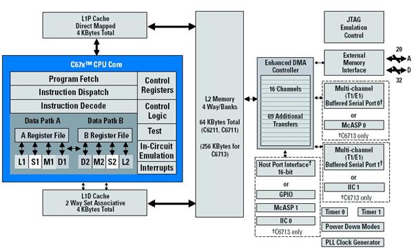
Figure 4‑2: The C67x DSPs’ two-level cache memory structure.

Applications

· Digital imaging

· Medical ultrasound

· Portable ultrasound equipment

· CT scanners

· Magnetic resonance imaging (Figure 4‑3)

Figure 4‑3: Magnetic Resonance Imaging implementation of TMS320C67 DSP.

4.9 Compiler Interface

As with modern DSPs, a C-compiler is provided to program and simulate the TMS32067x processor, so called Code Composer Studio. Using a compiler speeds and enhances the development process, and gives the ability to create and test real-time, embedded signal processing applications. C-compiler extends the capabilities to include full awareness of the DSP target by the host and real-time analysis tools. It’s user interface is shown in Figure 4‑4.

Figure 4‑4: User interface of C-compiler, Code Composer Studio.

5 Implementation

5.1 Introduction

Modern medical imaging devices provide ultra high-resolution data from the patient that is crucial for diagnosis. An example is Siemens Somatom (Figure 5‑1), which can produce informative 2048³ high resolution data. As the resolution increases, the data processing requirements increase as well. Real time interactive frame rates can be achieved at 33 Hz. minimum. This means 33 ´ 2048³ data cells should be visited every second and processed within a number of algorithms (Figure 5‑2). Such a speed is impossible to implement with software and conventional hardware. Special purpose hardware should be used as described in chapter 1.

Figure 5‑1: Medical data obtained from CT scanner.

Figure 5‑2: Reconstruction of three-dimensional data with high resolution.

A visualization process consists of three stages, that are, ray tracing, surface normal estimation, and shading. The latter two are applied to the final image obtained from the former. Therefore, the main part of this time-consuming process is ray tracing which is to be implemented with DSPs. Source code for this stage is given in next section.

5.2 Source Code

The C code for ray tracing is given below. VOX stands for voxel, the 3D data element which is represented by a coordinate triple such as (x, y, z) and its structure is as follows:

struct VOX

short x;

short y;

short z;

TEMP is the structure which holds ray template as explained in previous chapters. Every element of the template defines the difference on related axis that is necessary to move from one coordinate to the other in 3D discrete data space.

struct TEMP

int u_diff;

int v_diff;

int n_diff;

BASEWINDOW is the structure to hold the edge coordinates of the view plane (Figure 5‑3).

struct BASEWINDOW

VOX leftdown;

VOX leftup;

VOX rightdown;

VOX rightup;

Figure 5‑3: Structure BASEWINDOW and its relation with the view plane.

The variable “wcs_data” at line 39 holds the resolution of the dataset. The variable “vpw_data” at line 24 holds the 2D resolution of the view plane, that are the width and height of the plane.

Given the data with 3D resolution as (x_res, y_res, z_res), variable U at line 31 and variable V at line 29 holds x_res, and y_res respectively. Variable k in line 34 stands for z_res. It can be seen from the source code that every data element within the dataset is visited. Thus the loop between lines 29 and 55 runs x_res´y_res´z_res times which can be stated as the heart of the code.

The code between line 11 and 23 creates a ray template and loads to the memory, regarding to the projection specifications. This is achieved by the function “CreateRayTemplate”.

View plane is defined in a coordinate system, which is different from the data space. View plane is functioning as a camera. The data space is called “World Coordinate System (WC)” and the view plane space is called “View Reference Coordinate System (VRC)”. Since the edge coordinates of the view plane are defined in VRC within the structure BASEWINDOW, it needs to be transformed into WC prior to tracing process. This is achieved by the function “TransformVRCtoWC” at line 33.

int  RayTrace(BYTE * pdata)

1.                short axis, sayac, voxSayac, dU, dV;

2.                int U,V,numb_temp,k,val;

3.                int height=1; int width=1; int add;

4.                long offset, voxToplam;

5.                VOX vox, voxTmp, * fpCOOR;

6.                BYTE RGB, voxColor, * fpRGB;

7.                TEMP *temp;

8.                BASEWINDOW  Base;

9.                FILE * fpCOORraw, * fpRGBraw;

10.            int i,j;

11.            axis=FindAxis();

12.            basewdw=CalculateBaseWindow(axis);

13.            CreateRayTemplate();

14.            rewind(fp_ray_temp);

15.            fseek(fp_ray_temp,0,SEEK_END);

16.            offset=ftell(fp_ray_temp);

17.            numb_temp=offset/(3*sizeof(int));

18.            temp=(TEMP *) malloc(12 *  prwdw.time.ray_template);

19.            rewind(fp_ray_temp);

20.            for(k=0 ; k<prwdw.time.ray_template ; ++k)

21.            {

      fread(&temp[k],12,1,fp_ray_temp);

22.            }

23.            fclose(fp_ray_temp);

24.            dU=vpw_data.u_max - vpw_data.u_min;

25.            dV=vpw_data.v_max - vpw_data.v_min;

26.            fpbuf=(VOX *) calloc( dU * dV , sizeof(VOX) );

27.            fpCOOR=(VOX *) calloc( dU * dV , sizeof(VOX) );

28.            fpRGB=(BYTE *) calloc( dU * dV , sizeof(BYTE) );

29.            for(V=0 ; V < dV; ++V)

30.            {

31.                        for(U=0 ; U < dU ; ++U)

32.                        {

33.                                    voxTmp=TransformVRCtoWC(Base.x+U, Base.y+V, Base.z);

34.                                    for(k=0 ; k < numb_temp ; ++k)

35.                                    {

36.                                                ray_diff=temp[k];

37.                                                vox = voxTmp + ray_diff;

38.                                                voxTmp = vox;

39.                                                if(vox.x >= 0 && vox.y >= 0 && vox.z >= 0

                   && vox.x  < wcs_data.x && vox.y  < wcs_data.y &&

                   vox.z < wcs_data.z)

40.                                                {

41.                                                            val=calculate_address(vox.x,vox.y,vox.z);

42.                                                            if (val <0 or val > (totalfilesizeinbytes-3))break;

43.                                                            if( file[val] > treshold)

44.                                                            {

45.                                                                        RGB=file[val];

46.                                                                        pdata[CalculateOffsetIn256Bmp(U,V,dU)]=RGB;

47.                                                                        k=numb_temp+1;

48.                                                                        fpCOOR[U+(dU*V)]= vox;

49.                                                                        fpRGB[U+(dU*V)]= RGB;

50.                                                                        fpbuf[U+(dU*V)]=TransformWCtoVRC(vox.x,vox.y,vox.z);

51.                                                            }

52.                                                }

53.                                    }

54.                        }

55.            }

56.            free(temp);

57.            fpCOORraw=fopen("coorRT.tmp","w+b");

58.            fpRGBraw=fopen("rgbRT.tmp","w+b");

59.            for (i=0;i<(dU*dV);++i)

60.            {

61.                        fwrite(&fpCOOR[i],6L,1,fpCOORraw);

62.                        fwrite(&fpRGB[i],1L,1,fpRGBraw);

63.            }

64.            fclose(fpCOORraw);free(fpCOOR);

65.            fclose(fpRGBraw);free(fpRGB);

66.            return SUCCESS;

67.            }

References

[1] Levoy, M. (1988). Display of Surfaces from Volume Data. Computer Graphics and Applications, 8(5), 29-37.

[2] Knittel, G. (1993). VERVE-Voxel Engine for Real-Time Visualization and Examination. Eurographics ‘93, 12(3), 37- 48

[3] Günther, T., Poliwoda, C., Reinhart, C., Hesser, J., and Manner, J. (1994). VIRIM: A Massively Parallel Processor for Real-Time Volume Visualization in Medicine. Proceedings of the 9th Eurographics Hardware Workshop, 103-108

[4] Boer, M.De, Gröpl, A., Hesser, J., and Manner, R. (1996). Latency-and Hazard-free Volume Memory Architecture for Direct Volume Rendering. Eurographics Workshop on Graphics Hardware, 109-119

[5] Osborne, R., Pfister, H., Lauer, H., McKenzie, N., Gibson, S., Hiatt, W., and Ohkami, T. (1997). EM-Cube: An Architecture for Low-Cost Real-Time Volume Rendering. Proc. Eurographics/SIGGRAPH Workshop on Graphics Hardware, 131-138

[6] Dachille, F. (1997). Volume Visualization Algorithms and Architectures. Research Proficiency Exam, SUNY at Stony Brook

[7] Bakalash, R., Pfister, H., Kaufmann, A., and Pacheco, R. (1992). Cube-2: An Extended Volume Visualization System for Arbitrary Parallel Projection. In Proceedings of the 1992 Eurographics Workshop on Graphics Hardware Cambridge UK.

[8] Pfister, H., Kaufman, A., and Chiueh, T. (1994). Cube-3: A Real-Time Architecture for High-Resolution Volume Visualization. 1994 Workshop on Volume Visualization , 75-83

[9] Pfister, H., and Kaufman, A. (1995). Cube-4 : A scalable Architecture for Real-Time Volume Rendering. Technical Report TR-950115, Computer Science Department, SUNY at Stony Brook

[10] Kanus, U., Meissner, M., Strasser, W., Pfister, H., Kaufmann, A., Amerson, R., Carter, R.J., Culbertson, B., Kuekes, P., and Snider, G. (1997). Implementations of Cube-4 on the TERAMAC Custom Computing Machine. Computer and Graphics, 21(2), 199-208.

[11] Pfister, H., Hardenberg, J., Knittel, J., Lauer, H., and Seiler, L. (1999). The VolumePro Real-Time Ray-Casting System. SIGGRAPH 1999 Conference Proceedings, 251-260

[12] Texas Instruments TMS320C6713, TMS320C6713B Digital Signal Processors. Data sheet, Texas Instruments Inc., May 2004, Ver. SPRS1861