Chapter 11 Non-Parametric Techniques

  

  

  

11.1 Introduction

In maximum likelihood and Bayesian parameter estimation, we treated supervised learning under the assumption that the forms of the underlying density functions were known. In most pattern recognition applications, the common parametric forms rarely fit the densities actually encountered in practice. In particular, all of the classical paramet­ric densities are unimodal (have a single local maximum), whereas many practical problems involve multimodal densities. In this chapter, we shall examine nonparametric proce­dures that can be used with arbitrary distributions and without the assumption that the forms of the underlying densities are known.

  

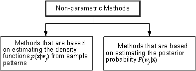
Figure 11.1: The classification of non-parametric methods in pattern recognition.

There are several types of nonparametric methods of interest in pattern recogni­tion (Figure 11.1 and Figure 11.2). One consists of procedures for estimating the density functions p(x|w_j) from sample patterns. If these estimates are satisfactory, they can be substituted for the true densities when designing the classifier. Another consists of procedures for directly estimating the posterior probabilities P(w_j|x). This is closely related to nonpara­metric design procedures such as the nearest-neighbor rule, which bypass probability estimation and go directly to decision functions

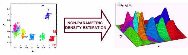
Figure 11.2: Non-parametric density estimation.

  

11.2 Density Estimation

The basic ideas behind many of the methods of estimating an unknown probability density function are very simple, and rely on the fact that the probability P that a vector x will fall in a region R is given by

                                                                                                                                                                               (11.1)

Thus P is a smoothed or averaged version of the density function p(x), and we can estimate this smoothed value of p by estimating the probability P. Suppose that n samples x₁,….,x_n are drawn independently and identically distributed (i.i.d.) according to the probability law p(x). Clearly, the probability that k of these n fall in R is given by the binomial law

                                                                                                                                                                            (11.2)

where

                                                                                                                                                                                                   (11.3)

and the expected value for k is

                                                                                                                                                                                                      (11.4)

Moreover, this binomial distribution for k peaks very sharply about the mean, so that we expect that the ratio k/n will be a very good estimate for the probability P, and hence for the smoothed density function. This estimate is especially accurate when n is very large. If we now assume that p(x) is continuous and that the region R. is so small that p does not vary appreciably within it, we can write

                                                                                                                                                                                                (11.5)

where x is a point within R, n is the total number of samples, k is the number of samples whose probability density function is to be estimated, and V is the volume enclosed by R Combining eqs.11.1,11.4, and 11.5, we arrive at the following obvious estimate for p(x),

                                                                                                                                                                                                          (11.6)

There are several problems that remain-some practical and some theoretical. If we fix the volume V and take more and more training samples, the ratio k/n will converge (in probability) as desired, but then we have only obtained an estimate of the space-averaged value of p(x),

                                                                                                                                                                               (11.7)

If we want to obtain p(x) rather than just an averaged version of it, we must be prepared to let V approach zero. However, if we fix the number n of samples and let V approach zero, the region will eventually become so small that it will enclose no samples, and our estimate p(x)@0 will be useless. Or if by chance one or more of the training samples coincide at x, the estimate diverges to infinity, which is equally useless.

From a practical standpoint, we note that the number of samples is always limited. Thus, the volume V cannot be allowed to become arbitrarily small. If this kind of estimate is to be used, one will have to accept a certain amount of variance in the ratio k/n and a certain amount of averaging of the density p(x).

From a theoretical standpoint, it is interesting to ask how these limitations can be circumvented if an unlimited number of samples is available. Suppose we use the following procedure. To estimate the density at x, we form a sequence of regions R₁, R₂,…, containing x-the first region to be used with one sample, the second with two, and so on. Let V_n  be the volume of R_n, k_n be the number of samples falling in R_n and p_n(x) be the n^th estimate for p(x):

                                                                                                                                                                               (11.8)

where

  

If p_n(x) is to converge to p(x), three conditions appear to be required:

1. : assures that the space averaged P/V will converge to p(x), if the size of the regions reduced uniformly and that p(.) is continuous at x

  : only makes sense if p(x)¹0, and assures that the frequency ratio will converge (in probability) to the probability P.       

     : necessary if p_n(x) is to converge at all. It also says that although a huge number of samples will eventually fall within the small region R_n, they will form a negligibly small fraction of the total number of samples

  

  

(a)

(b)

Figure 11.3: Non-parametric methods.

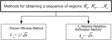
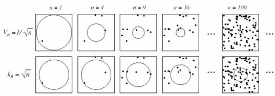
There are two common ways of obtaining sequences of regions that satisfy these conditions (Figure 11.3). One is to shrink an initial region by specifying the volume V_n as some function of n, such as V_n=. It then must be shown that the random variables k_n and k_n / n behave properly or, more to the point, that p_n(x) con­verges to p(x). This is basically, the Parzen-window method. The second method is to specify k_n, as some function of n, such as k_n =. Here the volume V_n, is grown until it encloses k_n neighbors of x. This is the k_n-nearest-neighbor estimation method. Both of these methods do in fact con­verge.

  

11.3 Parzen Windows

The Parzen-window approach to estimating densities can be introduced by temporar­ily assuming that. the region R_n is a d-dimensional hypercube which encloses k samples. If h_n is the length of an edge of that hypercube, then its volume is given by

                                                                                                                                                                                                      (11.9)

as shown in Figure 11.4.

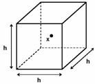
Figure 11.4: The hypercube defined by the region R.

  

We can obtain an analytic expression for k_n, the number of samples falling in the hypercube, by defining the following window function (kernel function):

                                                                                                                                              (11.10)

as shown in Figure 11.5.

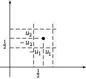
Figure 11.5: The kernel function in two dimensions.

  

Thus, j(u) defines a unit hypercube centered at the origin. It follows that j((x - x_i)/ h_n) is equal to unity if x_i falls within the hypercube of volume V_n, centered at x, and is zero otherwise. The number of samples in this hypercube is therefore given by

                                                                                                                                                                                                            (11.11)

as shown in Figure 11.6, and when we substitute this into eq.11.8 we obtain the estimate

                                                                                                                                                                                               (11.12)

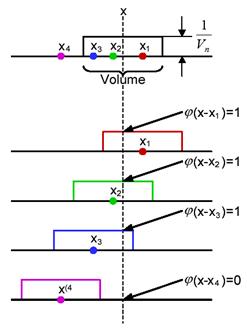
Figure 11.6: The calculation of number of samples within the kernel.

  

Equation 11.12 suggests a more general approach to estimating density functions. Rather than limiting ourselves to the hypercube window function of eq.11.10, suppose we allow a more general class of window functions. In such a case, eq.11.12 expresses our estimate for p(x) as an average of functions of x and the samples x_i. In essence, the window function is being used for interpolation—each sample contributing to the estimate in accordance with its distance from x.

It is natural to ask that the estimate p_n(x) be a legitimate density function, that is, that it be nonnegative and integrate to one. This can be assured by requiring the window function itself be a density function. To be more precise, if we require that

j(u) ³ 0                                                                                                                                                                                                                                                     (11.13)

and

                                                                                                                                                                                                                      (11.14)

and if we maintain the relation V_n =h, then it follows at once that p_n(x) also satisfies these conditions.

Let us examine the effect that the window width h_n has on p_n(x). If we define the function d_n(x) by

                                                                                                                                                                                                 (11.15)

then we can write p_n(x) as the average

                                                                                                                                                                            (11.16)

Because V_n =h, h_n clearly affects both the amplitude and the width of d_n(x) as shown in Figure 11.7. 

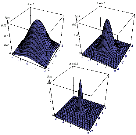
Figure 11.7: The effect of Parzen-Window width h_n on d (x).

If h_n is very large, then the amplitude of d_n is small, and x must be far from x_i before d_n(x- x_i) changes much from d_n(0). In this case, p_n(x) is the superposition of n broad, slowly changing functions and is a very smooth “out-of-focus” estimate of p(x). On the other hand, if h_n is very small, then the peak value of d_n(x- x_i) is large and occurs near x = x_i. In this case, p(x) is the superposition of n sharp pulses centered at the samples—a “noisy” estimate (Figure 11.9). For any value of h_n, the distribution is normalized, that is,

                                                                                                                                   (11.17)

Thus, as h_n approaches zero, d_n(x- x_i) approaches a Dirac delta function centered at x_i, and p_n(x) approaches a superposition of delta functions centered at the samples. 

The choice of h_n (or V_n) has an important effect on p_n(x) (Figure 11.8 and Figure 11.12). If V_n is too large, the estimate will suffer from too little resolution; if V_n is too small, the estimate will suffer from too much statistical variability. With a limited number of samples, the best we can do is to seek some acceptable compromise. However, with an unlimited number of samples, it is possible to let V_n slowly approach zero as n increases and have p_n(x) converge to the unknown density p(x).

  

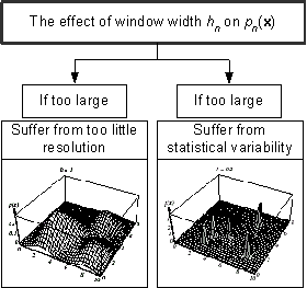
Figure 11.8: The effect of window width on the density function estimate.

  

In discussing convergence, we must recognize that we are talking about the con­vergence of a sequence of random variables, because for any fixed x the value of p_n(x) depends on the random samples x₁,….,x_n. Thus, p_n(x) has some mean (x) and variance . We shall say that the estimate p_n(x) converges to p(x) if

                                                                                                                                                                                                   (11.18)

and

                                                                                                                                                                                                                               (11.19)

  

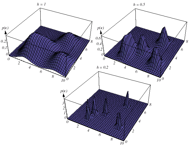
Figure 11.9: The effect of Parzen-window width h_n on the estimated density.

  

To prove convergence we must place conditions on the unknown density p(x), on the window function j(u), and on the window width h_n. In general, continuity of p(.) at x is required, and the conditions imposed by eqs.11.12 and 11.13 are customarily in­voked. Below we show that the following additional conditions assure convergence:

                                                                                                                                                                                                                                (11.20)

                                                                                                                                                                                                                        (11.21)

                                                                                                                                                                                                             (11.22)

and

                                                                                                                                                                                                          (11.23)

Equations 11.20 and 11.21 keep j(.) well behaved, and they are satisfied by most density functions that one might think of using for window functions. Equations 11.22 and 11.23 state that the volume V_n must approach zero, but at a rate slower than 1 / n. 

  

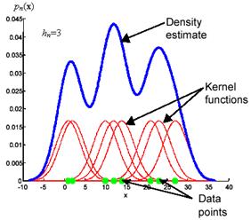
Figure 11.10: A simulation of how the Parzen-Window method works.

  

The Parzen window estimate can be considered as a sum of boxes centered at the observations, the smooth kernel estimate is a sum of boxes placed at the data points (Figure 11.10). The kernel function determines the shape of the boxes. The parameter h_n, also called the smoothing parameter or bandwidth, determines their width.

The problem of choosing the window width is crucial in density estimation. A large window width will over-smooth the density and mask the structure in the data. A small bandwidth will yield a density estimate that is spiky and very hard to interpret (Figure 11.11). We would like to find a value of the smoothing parameter that minimizes the error between the estimated density and the true density. A natural measure is the mean square error at the estimation point x. This expression is an example of the bias-variance tradeoff; the bias can be reduced at the expense of the variance, and vice versa. The bias of an estimate is the systematic error incurred in the estimation. The variance of an estimate is the random error incurred in the estimation. The bias-variance dilemma applied to window width selection simply means that; a large window width will reduce the differences among the estimates of density function for different data sets (the variance). A small window width will reduce the bias of density function, at the expense of a larger variance in the estimates of density function (Figure 11.12). 

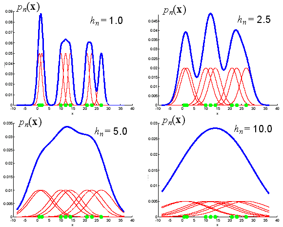
Figure 11.11: A simulation of the problem of choosing the window width.

  

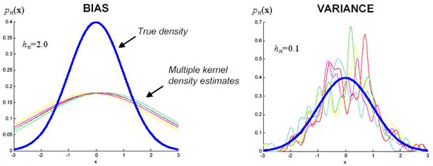
Figure 11.12: The bias-variance tradeoff.

11.3.1 Convergence of the Mean

Consider first , the mean of p_n(x). Because the samples x_i are independently drawn and identically distributed according to the (unknown) density p(x), we have

                               

          

           

                                                                                                                                                                          (11.24)

This equation shows that the expected value of the estimate is an averaged value of the unknown density-a convolution of the unknown density and the window function. Thus, is a blurred version of p(x) as seen through the averaging window. But as V_n approaches zero,  d_n(x-v) approaches a delta function centered at x. Thus, if p is continuous at x, eq.11.22 ensures that will approach p(x) as n approaches infinity.

  

11.3.2 Convergence of the Variance

Equation 11.24 shows that there is no need for an infinite number of samples to make approach p(x); one can achieve this for any n merely by letting V_n approach zero. Of course, for a particular set of n samples the resulting “spiky” estimate is useless; this fact highlights the need for us to consider the variance of the estimate. Because p_n(x) is the sum of functions of statistically independent random variables, its variance is the sum of the variances of the separate terms, and hence

   

        

                                                                                                                      (11.25)

By dropping the second term, bounding j (.) and using eq.11.24, we obtain

                                                                                                                                                                                         (11.26)

Clearly, to obtain a small variance we want a large value for V_n not a small one a large V_n smoothes out the local variations in density. However, because the numer­ator stays finite as n approaches infinity, we can let V_n  approach zero and still ob­tain zero variance, provided that nV_n approaches infinity. For example, we can let V_n= or inn or any other function satisfying eqs.11.22 and 11.23.

This is the principal theoretical result. Unfortunately, it does not tell us how to choose j (.) and V_n to obtain good results in the finite sample case. Indeed, unless we have more knowledge about p(x) than the mere fact that it is continuous, we have no direct basis for optimizing finite sample results.

  

11.3.3 Probabilistic Neural Networks (PNNs)

To show how the Parzen-window method can be implemented as a multilayer neural network known as a Probabilistic Neural Network is given in (Figure 11.13). The PNN is trained in the following way. First, each pattern x of the training set is normalized to have unit length, that is, scaled so that Sx=1. The first normalized training pattern is placed on the input units. The modifiable weights linking the input units and the first hidden unit are set such that w₁= x₁. (Note that because of the normalization of x₁, w₁ is normalized too.) Then, a single connection from the first hidden unit is made to the output unit corresponding to the known class of that pattern. The process is repeated with each of the remaining training patterns, setting the weights to the successive hidden units such that w_k= x_k for k = 1, 2…n. After such training, we have a network that is fully connected between input and hidden units, and sparsely connected from hidden to output units. If we denote the components of the j^th pattern as x_jk and the weights to the j^th hidden unit w_jk, for j = 1, 2…n and k = 1, 2…d, then our algorithm is as follows:

  

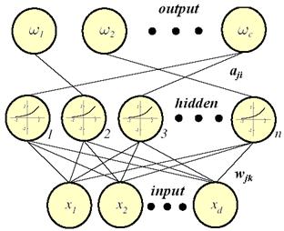
Figure 11.13: PNN implementation as multilayer neural network.

  

Algorithm (PNN Training)

begin initialize j ¬ 0, n, a_ji ¬ 0, for  j=1,…., n; i=1,…., c 

                                do                                           j ¬ j + 1 

                                                                                    x_jk  ¬  (normalize)

                                                                                                                w_jk  ¬  x_jk                            (train)

                                                            if x Îw_i then  a_ji ¬ 1

                until                     j = n

end

  

The trained network is then used for classification in the following way. A nor­malized test pattern x is placed at the input units. Each hidden unit computes the inner product to yield the net activation or simply net,

                                                                                                                                                                                                                       (11.27)

and emits a nonlinear function of net_k each output unit sums the contributions from all pattern units connected to it. The nonlinear function is , where s is a parameter set by the user and determines the width of the effective Gaussian win­dow. This activation function or transfer function, here must be an exponential to implement the Parzen windows algorithm. To see this, consider an (unnormalized) Gaussian window centered on the position of one of the training patterns w_k. We work backwards from the desired Gaussian window function to infer the nonlinear activation function that should be employed by the pattern units. That is, if we let our effective width h_n be a constant, the window function is

                                                       (11.28)

where we have used our normalization conditions x^Tx=ww_k=1. Thus, each pattern unit contributes to its associated category unit a signal equal to the proba­bility the test point was generated by a Gaussian centered on the associated training point. The sum of these local estimates (computed at the corresponding category unit) gives the discriminant function g_i(x) the Parzen-window estimate of the un­derlying distribution. The operation gives the desired category for the test point.

  

  

Algorithm (PNN Classification)

begin initialize k ¬ 0, n, x ¬ test pattern

                                do                                           k ¬ k + 1 (increment epoch)

                                                                                   

                                                                                                                w_jk  ¬  x_jk 

                                                            if a_ki = 1 then  g_i ¬ g_i +

                until                     k = n

                      return  

end

  

  

One of the benefits of PNNs is their speed of learning, because the learning rule (i.e., setting w_k= x_k) is simple and requires only a single pass through the training data. The space complexity (amount of memory) for the PNN is easy to determine by counting the number of connections. This can be quite se­vere for instance in a hardware application, because both n and d can be quite large. The time complexity for classification by the parallel implementation of Figure 11.13 is very low, since the n inner products of eq.11.29 can be done in parallel. Thus, this PNN architecture could find uses where recognition speed is important and storage is not a severe limitation. Another benefit is that new training patterns can be incorporated into a previously trained classifier quite easily; this might be important for a particu­lar on-line application.

  

11.3.4 Choosing the Window Function

As we have seen, one of the problems encountered in the Parzen-window/PNN ap­proach concerns the choice of the sequence of cell-volume sizes V₁,V₂…- or overall window size (or indeed other window parameters, such as shape or orientation). For example, if we take V_n=, the results for any finite n will be very sensitive to the choice for the initial volume V₁. If V₁ is too small, most of the volumes will be empty, and the estimate p_n(x) will be very erratic. On the other hand, if V₁ is too large, important spatial variations in p(x) may be lost due to averag­ing over the cell volume. Furthermore, it may well be the case that a cell volume appropriate for one region of the feature space might be entirely unsuitable in a dif­ferent region. General methods, including cross-validation, are often used in conjunction with Parzen windows. In brief, cross-validation requires taking some small portion of the data to form a validation set. The classifier is trained on the remaining patterns in the training set, but the window width is adjusted to give the smallest error on the validation set.

  

11.3.5 Estimation of Posterior Probabilities

These techniques can be used to estimate the pos­terior probabilities P(w_i|x) from a set of n labeled samples by using the samples to estimate the densities involved. Suppose that we place a cell of volume V around x and capture k samples, k_i of which turn out to be labeled w_i. Then the obvious estimate for the joint probability p(x ,w_i) is

                                                                                                                                                                                                  (11.29)

and thus a reasonable estimate for P(w_i|x) is

                                                                                                                                                                   (11.30)

That is, the estimate of the posterior probability that w_i is the state of nature is merely the fraction of the samples within the cell that are labeled w_i. Consequently, for minimum error rate we select the category most frequently represented within the cell. If there are enough samples and if the cell is sufficiently small, it can be shown that, this will yield performance approaching the best possible.

When it comes to choosing the size of the cell, it is clear that we can use either the Parzen-window approach or the k_n-nearest-neighbor approach. In the first case, V_n would be some specified function of n, such as V_n=l /. In the second case, V_n would be expanded until some specified number of samples were captured, such as k =. In either case, as n goes to infinity an infinite number of samples will fall within the infinitely small cell. The fact that the cell volume could become arbitrarily small and yet contain an arbitrarily large number of samples would allow us to learn the unknown probabilities with virtual certainty and thus eventually obtain optimum performance.

  

11.4 k_n – Nearest Neighbor Estimation

There are two overarching approaches to nonparametric estimation for pattern clas­sification: In one the densities are estimated (and then used for classification), while in the other the category is chosen directly. Parzen windows and their hardware implementation, probabilistic neural networks, exemplify the former approach. The latter is exemplified by k-nearest-neighbor and several forms of relaxation net­works.

A potential solution for the problem of the unknown best window function is to let the cell volume be a function of the training data, rather than some arbitrary function of the overall number of samples. For example, to estimate p(x) from training samples or prototypes we can center a cell about x and let it grow until it captures k_n samples, where k_n is some specified function of n. These samples are the k_n nearest-neighbors of x (Figure 11.14 and Figure 11.15).

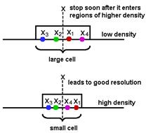
Figure 11.14: k_n-Nearest Neighbor estimation (kNN).

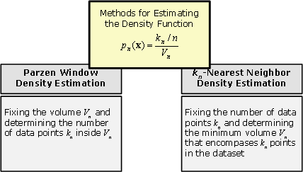
Figure 11.15: The difference between estimation methods for density function.

  

If the density is high near x (Figure 11.14), the cell will be relatively small, which leads to good resolution. If the density is low, it is true that the cell will grow large, but it will stop soon after it enters regions of higher density. In either case, if we take

                                                                                                                                                                                                       (11.31)

we want k_n to go to infinity as n goes to infinity, since this assures us that k_n / n will be a good estimate of the probability that a point will fall in the cell of volume V_n. However, we also want k_n to grow sufficiently slowly that the size of the cell needed to capture k_n training samples will shrink to zero. Thus, it is clear from eq.11.31 that the ratio k_n / n must go to zero. It can be shown that the conditions lim_n®¥ k_n =¥ and lim_n®¥ k_n/n=0 are necessary and sufficient for p_n(x) to converge to p(x) in probability at all points where p(x) is continuous. If we take k_n=and assume that p_n(x) is a reasonably good approximation to p(x), we then see from eq.11.31 that . Thus, V_n again has the form V₁/, but the initial volume V₁ is determined by the nature of the data rather than by some arbitrary choice on our part. Since p_n(x) is continuous, its slope is not, and the points of discontinuity are rarely the same as the data points (Figure 11.16).

If we base our decision solely on the label of the single nearest neighbor of x we can obtain comparable performance. We begin by letting Dⁿ={x₁,….,x_n} denote a set of n labeled prototypes (data point whose classes are known) and letting x¢Î Dⁿ be the prototype nearest to a test point x. Then the nearest-neighbor rule for classifying x is to assign it the label associated with x¢. The nearest-neighbor rule is a suboptimal procedure; its use will usually lead to an error rate greater than the minimum possible, the Bayes rate. With an unlimited number of prototypes, the error rate is never worse than twice the Bayes rate.

  

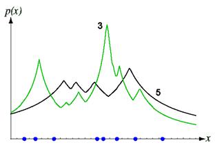
Figure 11.16: Eight points in one dimension and the k-nearest-neighbor density estimates, for k=3 and 5. The discontinuities in the slopes in the estimates generally lie away from the positions of the prototype points.

  

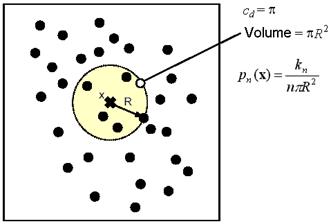
An extension of the nearest-neighbor rule is the k-nearest-neighbor rule. In the kNN method we grow the volume surrounding the estimation point x until it encloses a total of k_n data points.   This rule classifies x by assigning it the label most frequently represented among the k nearest samples; in other words, a deci­sion is made by examining the labels on the k nearest neighbors and taking a vote. The kNN query starts at the test point x and grows a spherical region until it encloses k training samples and it labels the test point by a majority vote of these samples. The density estimate then becomes;

                                                                                                                                                                                                       (11.32)

Since the volume is chosen to be spherical, the volume V_n can be written in terms of the volume of a unit sphere times the distance between the point x under estimate and the k_n nearest neighbor such as 

                                                                                                                                                                                                                   (11.33)

Combining eq. 11.32 and 11.33, the density estimation becomes 

                                                                                                                                                                                    (11.34)

where

The volume of the unit sphere c_d is given by

                                                                                                                                                                                                          (11.35)

where c₁=2, c₂=p, c₃=4p/3 and so on (Figure 11.17).

  

(a)                                                                                   (b)

Figure 11.17: a. The simulation of the k-nearest neighbor method, and b. k=5 case. In this case, the test point x would be labeled the category of the black points.

  

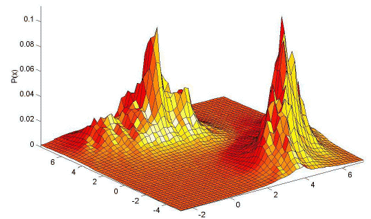
In general, the estimates that can be obtained with the kNN method are not very satisfactory. The estimates are prone to local noise. The method produces estimates with very heavy tails. Since the function R_k(x) is not differentiable, the density estimate will have discontinuities. The resulting density is not a true probability density since its integral over all the sample space diverges. These properties are illustrated in  Figure 11.18 and Figure 11.19.

  

(a)

(b)

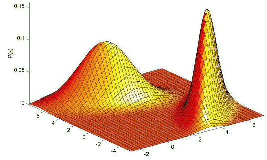
Figure 11.18: An illustration of the performance of k-nearest neighbor method. a. The true density which is a mixture of two bivariate Gaussians, and b. the density estimate for k=10 and n=200 examples.

(a)                                                                             (b)

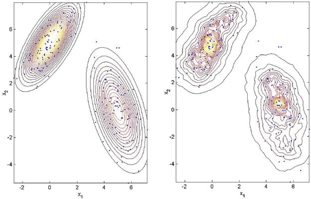
Figure 11.19: Contour plot of Figure 11.18. a. The true density, and b. the kNN density estimate.

  

The main advantage of the kNN method is that it leads to a very simple approximation of the (optimal) Bayes classifier. Assume that we have a dataset with n examples, n_i from class w_i, and that we are interested in classifying an unknown sample x_j. We draw a hyper-sphere of volume V around x_j. Assume this volume contains a total of k examples, k_i from class w_i. We can then approximate the likelihood functions using the kNN method by:

                                                                                                                                                                                                (11.36)

  

Similarly, the unconditional density is estimated by

                                                                                                                                                                                                         (11.37)

and the priors are approximated by

                                                                                                                                                                                                          (11.38)

Putting everything together, the Bayes classifier becomes

                                                                                                                                     (11.39)

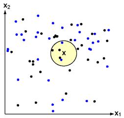
The k-Nearest Neighbor Rule (kNN) is a very intuitive method that classifies unlabeled examples based on their similarity to examples in the training set. For a given unlabeled example x_j, find the k “closest” labeled examples in the training data set and assign x_j to the class that appears most frequently within the k-subset. The kNN only requires;

·        An integer k,

·        A set of labeled examples (training data)

·        A metric to measure “closeness”

  

In the example in Figure 11.20, we have three classes and the goal is to find a class label for the unknown example x_j . In this case we use the Euclidean distance and a value of k=5 neighbors. Of the 5 closest neighbors, 4 belong to w₁ and 1 belongs to w₃, so x_j is assigned to w₁, the predominant class.   

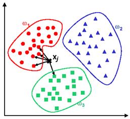
Figure 11.20: kNN classification example.

  

kNN is considered as a lazy learning algorithm. It defers data processing until it receives a request to classify an unlabelled example, replies to a request for information by combining its stored training data, and discards the constructed answer and any intermediate results.

Advantages:

·        Analytically tractable,

·        Simple implementation, 

·        Nearly optimal in the large sample limit (n ® ¥)

·        Uses local information, which can yield highly adaptive behavior, and

·        Lends itself very easily to parallel implementations.

  

Disadvantages:

·        Large storage requirements,

·        Computationally intensive recall,

·        Highly susceptible to the curse of dimensionality.

  

11.5 MATLAB Implementation

The probabilistic neural network and the classification algorithm is simulated using MATLAB. The network used for this demonstration is shown in Figure 11.21. Given the samples of three different classes as shown in Figure 11.22, the training is implemented, and then, a new sample is presented to the network for classification as shown in Figure 11.23. The PNN actually divides the input space into three classes as shown in Figure 11.24.

Matlab script: ccPnn.m 

  

  

  

  

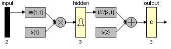
Figure 11.21: The PNN structure used for the classification example.

  

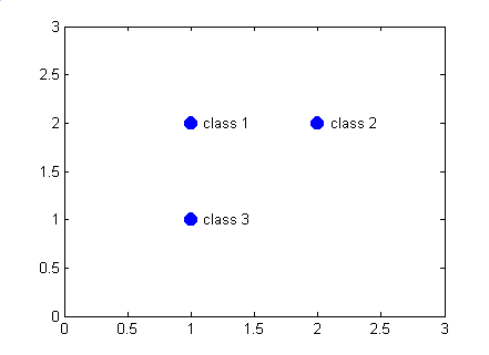
Figure 11.22: The PNN structure used for the classification example.

  

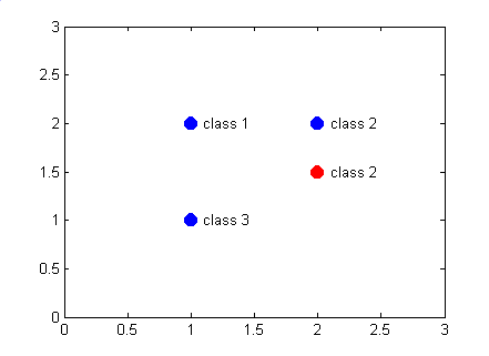
Figure 11.23: The PNN structure used for the classification example.

  

  

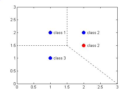
Figure 11.24: The PNN structure used for the classification example.

  

  

  

REFERENCES

  

[1]               Duda, R.O., Hart, P.E., and Stork D.G., (2001). Pattern Classification. (2^nd ed.). New York: Wiley-Interscience Publication.

[2]               Neural Network Toolbox For Use With MATLAB, User’s Guide, (2003) Mathworks Inc., ver.4.0

[3]               Gutierrez-Osuna R., Introduction to Pattern Analysis, Course Notes, Department of Computer Science, A&M University, Texas

[4]               Sima J. (1998). Introduction to Neural Networks, Technical Report No. V 755, Institute of Computer Science, Academy of Sciences of the Czech Republic

[5]               Kröse B., and van der Smagt P. (1996). An Introduction to Neural Networks. (8^th ed.) University of Amsterdam Press, University of Amsterdam.

[6]               Gurney K. (1997). An Introduction to Neural Networks. (1^st ed.) UCL Press, London EC4A 3DE, UK.

[7]               Paplinski A.P. Neural Nets. Lecture Notes, Dept. of Computer Sciences, and Software Eng., Manash University, Clayton-AUSTRALIA

[8]               Bain J. L, and Engelhardt M. (1991) Introduction to Probability and Mathematical Statistics. (2^nd ed.), Duxbury Publication, California-USA