The class of solutions that can be obtained from networks that implements linear discriminant functions is not general enough in demanding applications: there are many problems for which linear discriminants are insufficient for minimum error. With a clever choice of nonlinear functions, however, we can obtain arbitrary decision regions. The central difficulty is choosing the appropriate nonlinear functions. Multilayer neural networks learn the nonlinearity at the same time as the linear discriminant. They implement linear discriminants in a space where the inputs have been mapped nonlinearly. They admit simple algorithms where the form of the nonlinearity can be learned from training data.
Figure 10.1: A simple three-layer neural network.
Figure 10.1 shows a simple three-layer neural network, which consists of an input layer, a hidden layer, and an output layer, interconnected by modifiable weights, represented by links between layers. There is a single bias unit, which is connected to each unit other than the input units. Each two-dimensional input vector is presented to the input layer, and the output of each input unit equals the corresponding component in the vector. Each hidden unit computes the weighted sum of its inputs to form its scalar net activation, which is denoted simply as net. That is, the net activation is the inner product of the inputs with the weights at the hidden unit. Thus, it can be written
![]() (10.1)
(10.1)
where the subscript i indexes units in the input layer, j in the hidden; wji denotes the input-to-hidden layer weights at the hidden unit j. Each hidden unit emits an output that is a nonlinear function of its activation, f(net), that is,
yj=f(netj) (10.2)
Figure 10.1 shows a simple threshold or sign (read “signum”) function,
![]() (10.3)
(10.3)
but other functions have more desirable properties and are hence more commonly used. This f(.) is called the activation function or nonlinearity of a unit. Each output unit computes its net activation based on the hidden unit signals as
![]() (10.4)
(10.4)
where the subscript k indexes units in the output layer and nH denotes the number of hidden units. We have mathematically treated the bias unit as equivalent to one of the hidden units whose output is always y 0 =1. In this example, there is only one output unit. However, anticipating a more general case, we shall refer to its output as zk . An output unit computes the nonlinear function of its net, emitting
zk=f(netk) (10.5)
The output zk can also be thought of as a function of the input feature vector x. When there are c output units, we can think of the network as computing c discriminant functions zk=g(x), and can classify the input according to which discriminant function is largest. In a two-category case, it is traditional to use a single output unit and label a pattern by the sign of the output z.
This discussion can be generalized to more inputs, other nonlinearities, and arbitrary number of output units. For classification, we will have c output units, one for each of the categories, and the signal from each output unit is the discriminant function gk(x). We gather the results from eqs. 10.1, 10.2, 10.4, and 10.5, to express such discriminant functions as
 (10.6)
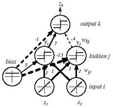
This, then, is the class of functions that can be implemented by a three-layer neural network. In general, the activation function does not have to be a sign function. Indeed, it is often required the activation functions to be continuous and differentiable. We can even allow the activation functions in the output layer to be different from the activation functions in the hidden layer, or indeed have different activation functions for each individual unit. Figure 10.2 shows a three-layer network and the notation that is used in this text.
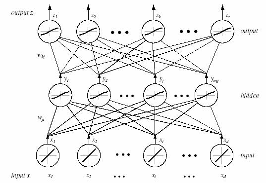
Figure 10.2: A three-layer neural network and the notation used.
Setting the weights based on training patterns and the desired output is the crucial problem. The backpropagation is one of the simplest and most general methods for supervised training of multilayer neural networks. Nevertheless, how should the input-to-hidden weights be learned, the ones governing the nonlinear transformation of the input vectors? If the “proper” outputs for a hidden unit were known for any pattern, the input-to-hidden weights could be adjusted to approximate it. However, there is no explicit teacher to state what the hidden unit’s output should be. This is called the credit assignment problem. Back-propagation allows us to calculate an effective error for each hidden unit, and thus derive a learning rule for the input-to-hidden weights.
Networks have two primary modes of operation: feedforward and learning. Feed-forward operation consists of presenting a pattern to the input units and passing the signals through the network in order to yield outputs from the output units. Supervised learning consists of presenting an input pattern and changing the network parameters to bring the actual outputs closer to the desired teaching or target values.
The basic approach in learning is to start with an untrained network, present a training pattern to the input layer, pass the signals through the net and determine the output at the output layer. Here these outputs are compared to the target values; any difference corresponds to an error. This error or criterion function is some scalar function of the weights and is minimized when the network outputs match the desired outputs. Thus, the weights are adjusted to reduce this measure of error.
We consider the training error on a pattern to be the sum over output units of the squared difference between the desired output tk given by a teacher and the actual output zk:
![]() (10.7)
(10.7)
where t and z are the target and the network output vectors of length c and w represents all the weights in the network.
The backpropagation learning rule is based on gradient descent. The weights are initialized with random values, and then they are changed in a direction that will reduce the error:
![]() (10.8)
(10.8)
or in component form
![]() (10.9)
(10.9)
where h is the learning rate, and indicates the relative size of the change in weights. Eqs. 10.8 and 10.9 demand that we take a step in weight space that lowers the criterion function. It is clear from eq.10.7 that the criterion function can never be negative; the learning rule guarantees that learning will stop. This iterative algorithm requires taking a weight vector at iteration m and updating it as
![]() (10.10)
(10.10)
where m indexes the particular pattern presentation.
We now turn to the problem of evaluating eq.10.9 for a three-layer net. Consider first the hidden-to-output weights, wij . Because the error is not explicitly dependent upon wjk , we must use the chain rule for differentiation:
![]() (10.11)
(10.11)
where the sensitivity of unit k is defined to be
![]() (10.12)
(10.12)
and describes how the overall error changes with the unit’s net activation and determines the direction of search in weight space for the weights . Assuming that the activation function f(.) is differentiable, we differentiate eq. 10.7 and find that for such an output unit, d k is simply
![]() (10.13)
(10.13)
The last derivative in eq. 10.11 is found using eq.10.4:
![]() (10.14)
(10.14)
Taken together, these results give the weight update or learning rule for the hidden-to-output weights:
![]() (10.15)
(10.15)
The learning rule for the input-to-hidden units is subtle; indeed, it is the central point of the solution to the credit assignment problem. From eq. 10.9, and again using the chain rule, we calculate
![]() (10.16)
(10.16)
The first term on the right-hand side involves all of the weights wkj , and requires just a bit of care:
![]()
![]()
![]()
![]() (10.17)
(10.17)
For the second step above, we had to use the chain rule yet again. The final sum over output units in eq.10.17 expresses how the hidden unit output yj, affects the error at each output unit. This will allow us to compute an effective target activiation for each hidden unit. With eq.10.13 we use eq.10.17 to define the sensitivity for a hidden unit as
![]() (10.18)
(10.18)
Equation 10.18 is the core of the solution to the credit assignment problem: The sensitivity at a hidden unit is simply the sum of the individual sensitivities at the output units weighted by the hidden-to-output weights wkj , all multiplied by f ¢ (netj). Thus the learning rule for the input-to-hidden weights is
 (10.19)
Equations 10.15 and 10.19, together with training protocols described below, give the backpropagation algorithm, or more specifically the “backpropagation of errors” algorithm. It is so-called because during training an error must be propagated from the output layer back to the hidden layer in order to perform the learning of the input-to-hidden weights by eq. 10.19 (Figure 10.3). At base then, backpropagation is just gradient descent in layered models where application of the chain rule through continuous functions allows the computation of derivatives of the criterion function with respect to all model weights.
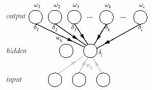
Figure 10.3: The sensitivity at a hidden unit is proportional to the weighted sum of the sensitivities at the output units. The output unit sensitivities are propagated back to the hidden units.
As with all gradient-descent procedures, the exact behavior of the backpropagation algorithm depends on the starting point. While it might seem natural to start by setting the weight values to 0, eq.10.19 reveals that that would have very undesirable consequences. If the weights wkj to the output layer were ever all zero, the back-propagated error would also be zero and the input-to-hidden weights would never change. This is the reason we start the process with random values for weights.
These learning rules make intuitive sense. Consider first the rule for learning weights at the output units (eq.10.15). The weight update at unit k should indeed be proportional to (tk - zk): If we get the desired output ( zk = tk ), then there should be no weight change. For the typical sigmoid f(.) we shall use most often, f’ ( netk ) is always positive. Thus if yj and ( t k - zk) are both positive, then the actual output is too small and the weight must be increased; indeed, the proper sign is given by the learning rule. Finally, the weight update should be proportional to the input value; if yj = 0, then hidden unit j has no effect on the output and hence the error, and thus changing wji , will not change the error on the pattern presented. A similar analysis of eq.10.19 yields insight of the input-to-hidden weights.
Although this analysis was done for a special case of a particularly simple three-layer network, it can readily be extended to much more general networks. The back-propagation-learning algorithm can be generalized directly to feed-forward networks in which
• Input units include a bias unit.
• Input units are connected directly to output units as well as to hidden units.
• There are more than three layers of units.
• There are different nonlinearities for different layers.
• Each unit has its own nonlinearity.
• Each unit has a different learning rate.
We describe the overall amount of pattern presentations by epoch—where one epoch corresponds to a single presentations of all patterns in the training set. For other variables being constant, the number of epochs is an indication of the relative amount of learning.
The three most useful training protocols are: stochastic, batch, and on-line. All of the three algorithms end when the change in the criterion function J(w) is smaller than some preset value q . While this is perhaps the simplest meaningful stopping criterion, others generally lead to better performance.
Stochastic Backpropagation Algorithm: In stochastic training patterns are chosen randomly from the training set, and the network weights are updated for each pattern presentation. This method is called stochastic because the training data can be considered a random variable. In stochastic training, a weight update may reduce the error on the single pattern being presented, yet increase the error on the full training set. Given a large number of such individual updates, however, the total error as given in eq.10.20 decreases.
Algorithm (Stochastic Backpropagation)
begin initialize n H , w , criterion q , h , m ¬ 0
do m ¬ m + 1
xm ¬ randomly chosen pattern
wji
¬ wji +
![]() ; wkj¬
wkj
+
; wkj¬
wkj
+
![]()
until
![]()
return w
end
On-Line Backpropagation Algorithm: In on- line training , each pattern is presented once and only once; there is no use of memory for storing the patterns.
Algorithm (On-Line Backpropagation)
begin initialize n H , w , criterion q , h , m ¬ 0
do m ¬ m + 1
xm ¬ sequentially chosen pattern
wji
¬ wji +
![]() ; wkj¬
wkj
+
; wkj¬
wkj
+
![]()
until
![]()
return w
end
Batch Backpropagation Algorithm: In batch training, all patterns are presented to the network before learning takes place. In virtually every case we must make several passes through the training data. In the batch training protocol, all the training patterns are presented first and their corresponding weight updates summed; only then are the actual weights in the network updated. This process is iterated until some stopping criterion is met. In batch backpropagation, we need not select patterns randomly, because the weights are updated only after all patterns have been presented once.
Algorithm (Batch Backpropagation)
begin initialize n H , w , criterion q , h , r ¬ 0
do r ¬ r + 1 (increment epoch)
m ¬ 0 ; D wji ¬ 0; D wkj ¬ 0
do m ¬ m + 1
xm ¬ select pattern
Dwji¬
Dwji +
![]() ; D
wkj
¬ Dwkj +
; D
wkj
¬ Dwkj +
![]()
until m=n
wji ¬ wji +Dwji; wkj¬ wkj +Dwkj
until
![]()
return w
end
So far we have considered the error on a single pattern, but in fact we want to consider an error defined over the entirety of patterns in the training set. While we have to be careful about ambiguities in notation, we can nevertheless write this total training error as the sum over the errors on n individual patterns:
![]() (10.20)
(10.20)
Before training has begun, the error on the training set is typically high; through learning, the error becomes lower, as shown in a learning curve (Figure 10.4). The (per pattern) training error reaches an asymptotic value which depends upon the Bayes error, the amount of training data, and the number of weights in the network: The higher the Bayes error and the fewer the number of such weights, the higher this asymptotic value is likely to be. Because batch back-propagation performs gradient descent in the criterion function, if the learning rate is not too high, the training error tends to decrease monotonically. The average error on an independent test set is always higher than on the training set, and while it generally decreases, it can increase or oscillate.
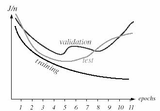
Figure 10.4: Learning curve and its relation with validation and test sets.
In addition to the use of the training set, there are two conceptual uses of independently selected patterns. One is to state the performance of the fielded network; for this we use the test set. Another use is to decide when to stop training ; for this we use a validation set. We stop training at a minimum of the error on the validation set.
In general, back-propagation algorithm cannot be shown to convergence, and there are no well-defined criteria for stopping its operation. Rather there are some reasonable criteria, each with its own practical merit, which may be used to terminate the weight adjustments. It is logical to think in terms of the unique properties of a local or global minimum of the error surface. Figure 10.4 also shows the average error on a validation set-patterns not used directly for gradient descent training, and thus indirectly representative of novel patterns yet to be classified. The validation set can be used in a stopping criterion in both batch and stochastic protocols; gradient descent learning of the training set is stopped when a minimum is reached in the validation error (e.g., near epoch 5 in the figure). Here are two stopping criteria are stated below:
1. The back-propagation algorithm is considered to have converged when the Euclidean norm of the gradient vector reaches a sufficiently small gradient threshold.
2. The back-propagation algorithm is considered to have converged when the absolute rate of change in the average squared error per epoch is sufficiently small.
The function J(w) provides us a tool which can be studied to find a local minima. It is called error surface. Such an error surface depends upon the classification task. There are some general properties of error surfaces that hold over a broad range of real-world pattern recognition problems. In order to obtain an error surface, plot the error against weight values. Consider the network as a function that returns an error. Each connection weight is one parameter of this function. Low points in surface are considered as local minima and the lowest is the global minimum (Figure 10.5).
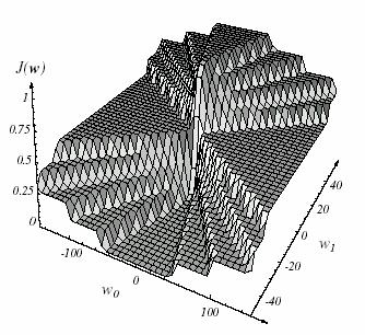
Figure 10.5: The error surface as a function of w0 and w1 in a linearly separable one-dimensional pattern.
The possibility of the presence of multiple local minima is one reason that we resort to iterative gradient descent-analytic methods are highly unlikely to find a single global minimum, especially in high-dimensional weight spaces. In computational practice, we do not want our network to be caught in a local minimum having high training error because this usually indicates that key features of the problem have not been learned by the network. In such cases, it is traditional to reinitialize the weights and train again, possibly also altering other parameters in the net.
In many problems, convergence to a non-global minimum is acceptable, if the error is fairly low. Furthermore, common stopping criteria demand that training terminate even before the minimum is reached, and thus it is not essential that the network be converging toward the global minimum for acceptable performance. In short, the presence of multiple minima does not necessarily present difficulties in training nets.
Hidden neurons play a critical role in the operation of a multilayer network with back-propagation learning because they act as feature detectors. As the learning process progresses, the hidden neurons begin to gradually discover the considerable features that characterize the training data. They do so by performing a nonlinear transformation on the input data into a new space called the hidden space, or feature space. In this new space the classes of interest in a pattern classification task, may be more easily separated from each other than in the original input space.
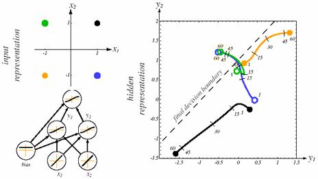
Figure 10.6: Feature mapping with hidden units.
Figure 10.6 shows a three-layer net addressing the XOR problem. For any input pattern in the x1x2-space, we can show the corresponding output of the two hidden units in the y1y2-space. With small initial weights, the net activation of each hidden unit is small, and thus the linear portion of their activation function is used. Such a linear transformation from x to y leaves the patterns linearly inseparable. However, as learning progresses and the input-to-hidden weights increase in magnitude, the nonlinearities of the hidden units warp and distort the mapping from input to the hidden unit space. The linear decision boundary at the end of learning found by the hidden-to-output weights is shown by the straight dashed line; the nonlinearly separable problem at the inputs is transformed into a linearly separable at the hidden units.
In addition to visualizing on the transformation of patterns in a network, we can also consider the representation of learned weights. Because the hidden-to-output weighs merely leads to a linear discriminant, it is instead the input-to-hidden weights that are most instructive. In particular, such weights at a single hidden unit describe the input pattern that leads to maximum activation of that hidden unit. It is convenient to think of the hidden units as finding feature groupings useful for the linear classifier implemented by the hidden-to-output layer weights.
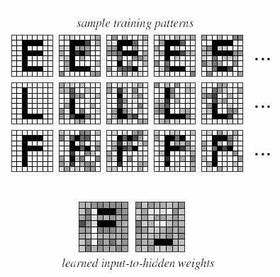
Figure 10.7: Representation at the hidden layer.
Figure 10.7 shows the input-to-hidden weights, displayed as images, for a simple task of character recognition. One hidden unit seems “tuned” or “matched” to a pair of horizontal bars while the other is tuned to a single lower bar. Both of these feature groupings are useful building blocks for the patterns presented. In complex, high-dimensional problems, the pattern of learned weights may not appear to be simply related to the features we suspect are appropriate for the task. This could be because we may be mistaken about which are the true, relevant feature groupings; nonlinear interactions between features may be significant in a problem and such interactions are not manifest in the patterns of weights at a single hidden unit; or the network may have too many weights, and thus the feature selectivity is low. Thus, while analyses of learned weights may be suggestive, the whole endeavor must be approached with caution.
When multilayer neural networks are trained via backpropagation on a sum-squared error criterion, they provide a least squares fit to the Bayes discriminant functions. The LMS algorithm computed the approximation to the Bayes discriminant function for two-layer nets. Now this result can be generalized in two ways: to multiple categories and to nonlinear functions implemented by three-layer neural networks. Let gk(x; w) be the output of the kth output unit-the discriminant function corresponding to category wk . . Recall Bayes formula,
 (10.21)
and the Bayes decision for any pattern x: Choose the category wk having the largest discriminant function gk(x)=P(wk|x).
Suppose we train a network having c output units with a target signal according to
![]() (10.22)
(10.22)
The contribution to the criterion function based on a single output unit k for finite number of training samples x is
![]() (10.23)
(10.23)
![]()

where n is the total number of training patterns, nk of which are in wk . . In the limit of infinite data, we can use Bayes formula to express eq.10.23 as
![]() (10.24)
(10.24)
![]()
![]()
![]()
The backpropagation rule changes weights to minimize the left-hand side of eq.10.24, and thus it minimizes
![]() (10.25)
(10.25)
Because this is true for each category wk (k = 1, 2,..., c ), backpropagation minimizes the sum:
![]() (10.26)
(10.26)
Thus, in the limit of infinite data, the outputs of the trained network will approximate the true posterior probabilities in a least-squares sense; that is, the output units represent the posterior probabilities,
![]() (10.27)
(10.27)
We must be cautious in interpreting these results, however. A key assumption underlying the argument is that the network can indeed represent the functions P(wk|x); with insufficient hidden units, this will not be true. Nevertheless, the above results show that neural networks can have very desirable limiting properties.
While indeed given infinite amounts of training data, the outputs will represent probabilities. If, however, these conditions do not hold-in particular we have only a finite amount of training data-then the outputs will not represent probabilities; for instance, there is not even a guarantee that they sum to 1. In fact, if the sum of the network outputs differs significantly from 1 within some range of the input space, it is an indication that the network is not accurately modeling the posteriors. This, in turn, may suggest changing the network topology, number of hidden units, or other aspects of the net.
One approach toward
approximating probabilities is to choose the output unit nonlinearity to be
exponential rather than sigmoidal-
f
(netk)
a
![]() -and for each pattern to normalize the outputs to sum to 1,
-and for each pattern to normalize the outputs to sum to 1,
 (10.28)
while training using 0-1 target signals. This is the softmax method a smoothed or continuous version of a winner-take-all nonlinearity in which the maximum output is transformed to 1, and all others reduced to 0.0. The softmax output finds theoretical justification if for each category wk the hidden unit representations y can be assumed to come from an exponential distribution.
As we have seen, then, a neural network classifier trained in this manner approximates the posterior probabilities P(wi|x), and this depends upon the prior probabilities of the categories. If such a trained network is to be used on problems in which the priors have been changed, it is a simple matter to rescale each network output, gi(x)=P(wi|x), by the ratio of such priors. The use of softmax is appropriate when the network is to be used for estimating probabilities. While probabilities as network outputs can certainly be used for classification, other representations-for instance, where outputs can be positive or negative and need not sum to 1 are preferable.
Although the above analyses are correct, a naive application of the procedures can lead to very slow convergence, poor performance or other unsatisfactory results. Thus, we now turn to a number of practical suggestions for training networks by backpropagation, which have been found to be useful in many practical applications. Most of the heuristics described below can be used alone or in combination. While they may interact in unexpected ways, all have found use in important pattern recognition problems and classifier designers should have experience with all of them.
Backpropagation will work with virtually any activation function, given that a few simple conditions such as continuity of f(.) and its derivative are met. For instance, if we have prior information that the distributions arise from a mixture of Gaussians, then Gaussian activation functions are appropriate. In any given classification problem we may have a good reason for selecting a particular activation function.
There are a number of properties we seek for f(.):
1. f(.) must be nonlinear: otherwise the three-layer network provides no computational power above that of a two-layer net
2. f(.) saturate : that is, have some maximum and minimum output value. This will keep the weights and activations bounded, and thus keep the training time limited. Saturation is a particularly desirable property when the output is meant to represent a probability. It is also desirable for models of biological neural networks, where the output represents a neural firing rate. It may not be desirable in networks used for regression, where a wide dynamic range may be required.
3. continuity and smoothness: that is, that f(.) and f’(.) be defined throughout the range of their argument. Recall that the fact that we could take a derivative of f(.) was crucial in the derivation of the backpropagation learning rule. The rule would not, therefore, work with the threshold or sign function of Eq. 3. Backpropagation can be made to work with piecewise linear activation functions, but with added complexity and few benefits.
4. monotonicity : convenient, but nonessential, property for f(.)-we might wish that the derivative have the same sign throughout the range of the argument, for example, f’(.) ³0. If f is not monotonic and has multiple local maxima, additional and undesirable local extrema in the error surface may become introduced. Non-monotonic activation functions such as radial basis functions can be used if proper care is taken.
5. linearity : for a small value of net, which will enable the system to implement a linear model if adequate for yielding low error.
One class of functions that has all the above desired properties is the sigmoid, such as a hyperbolic tangent. The sigmoid is smooth, differentiable, nonlinear, and saturating, thus, is the most widely used activation function.
Given that we will use the sigmoidal activation function, there remain a number of parameters to set. It is best to keep the function centered on zero and anti-symmetric-or as an “odd” function, that is, f(-net)= -f(net) -rather than one whose valor is always positive. Together with the data preprocessing, anti-symmetric sigmoids lead to faster learning. Nonzero means in the input variable and activation functions make some of the eigenvalues of the Hessian matrix large, and this slows the learning. Sigmoid functions of the form
![]() (10.29)
(10.29)
work well. The overall range and slope are not important, because it is their relationship to parameters such as the learning rate and magnitudes of the inputs and targets that affect learning. For convenience, we choose a = 1.716 and b = 2/3 in eq.10.29 values that ensure f’(0) @0.5, that the linear range is -1< net < +1, and that the extrema of the second derivative occur roughly at net @ ± 2.
Suppose we were using a two-input network to classify fish based on the features of mass (measured in grams) and length (measured in meters). Such a representation will have serious drawbacks for a neural network classifier: The numerical value of the mass will be orders of magnitude larger than that for length. During training, the network will adjust weights from the “mass” input unit far more than for the “length” input-indeed the error will hardly depend upon the tiny length values. If, however the same physical information were presented but with mass measured in kilograms and length in millimeters, the situation would be reversed. Naturally, we do not want our classifier to prefer one of these features over the other, because they differ solely in the arbitrary representation. The difficulty arises even for features having the same units but differing in overall magnitude, of course-for instance, if a fish’s length and its fin thickness were both measured in millimeters.
In order to avoid such difficulties, the input patterns should be shifted so that the average over the training set of each feature is zero. Moreover, the full data set should then be scaled to have the same variance in each feature component-here chosen to be 1.0. That is, we standardize the training patterns. This data standardization need be done once, before the start of network training. It represents a small one-time computational burden. Standardization can only be done for stochastic and batch learning protocols, but not on-line protocols where the full data set is never available at any one time. Naturally, any test pattern must be subjected to the same transformation before it is to be classified by the network.
For pattern recognition, we typically train with the pattern and its category label, and thus we use a one-of-c representation for the target vector. Because the output units saturate at ± 1.716, we might naively feel that the target values should be those values; however, that would present a difficulty. For any finite value of netk , the output could never reach these saturation values, and thus there would be error. Full training would never terminate because weights would become extremely large, as netk would be driven to + ¥ . This difficulty can be avoided by using teaching values of +1 for the target category and -1 for the non-target categories. For instance, in a four-category problem if the pattern is in category W3, the following target vector should be used: t = (-1, -1, +1, -1) T Of course, this target representation yields efficient learning for categorization-the outputs here do not represent posterior probabilities.
When the training set is small, one can generate virtual training pattern and use them as if they were normal training patterns sampled from the source distributions. In the absence of problem-specific information, a natural assumption is that such virtual patterns should be made by adding d-dimensional Gaussian noise to true training points. In particular, for the standardized inputs, described in Section 10.5.3, the variance of the added noise should be less than 1.0 (e.g., 0.1) and the category label should be left unchanged. This method of training with noise can be used with virtually every classification method, though it generally does not improve accuracy for highly local classifiers such as ones based on the nearest neighbor.
If we have knowledge about the sources of variation among patterns, for instance, due to geometrical invariances, we can “manufacture” training data that conveys more information than does the method of training with uncorrelated noise (Section 10.5.5). For instance, in an optical character recognition problem, an input image’ may be presented rotated by various amounts. Hence, during training we can take any particular training pattern and rotate its image to “manufacture” a training point that may be representative of a much larger training set. Likewise, we might scale a pattern, perform simple image processing to simulate a bold face character, and so on. If we have information about the range of expected rotation angles, or the variation in thickness of the character strokes, we should manufacture the data accordingly.
While this method bears formal equivalence to incorporating prior information in a maximum-likelihood approach, it is usually much simpler to implement, because we need only the forward model for generating patterns. As with training with noise, manufacturing data can be used with a wide range of pattern recognition methods, A drawback is that the memory requirements may be large and overall training may be slow.
While the number of input units and output units are dictated by the dimensionality of the input vectors and the number of categories, respectively, the number of hidden units is not simply related to such obvious properties of the classification problem. The number of hidden units, nH governs the expressive power of the net-and thus the complexity of the decision boundary. If the patterns are well separated or linearly separable, then few hidden units are needed; conversely, if the patterns are drawn from complicated densities that are highly interspersed, then more hidden units are needed. Without further information, there is no foolproof method for setting the number of hidden units before training.
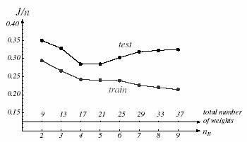
Figure 10.8: The error per pattern for networks fully trained but differing in the number of hidden units.
Figure 10.8 shows the training and test error on a two-category classification problem for networks that differ in their number of hidden units. For large nH, the training error can become small because such networks have high expressive power and become tuned to the particular training set. Nevertheless, in this method, the test error is unacceptably high. At the other extreme of too few hidden units, the net does not have enough free parameters to fit the training data well, and again the test error is high. We seek some intermediate number of hidden units that will give low test error.
The number of hidden units determines the total number of weights in the net, which we consider informally as the number of degrees of freedom-and we should not have more weights than the total number of training points, n. A convenient rule is to choose the number of hidden units such that the total number of weights in the net is roughly n/10. This seems to work well over a range of practical problems. It must be noted that many successful systems employ more than this number. A more principled method is to adjust the complexity of the network in response to the training data, for instance, start with a “large” number of hidden units and “decay,” prune, or eliminate weights-techniques.
We cannot initialize the weights to 0, otherwise learning cannot take place. Thus, we must confront the problem of choosing their starting values. Suppose we have fixed the network topology and thus have set the number of hidden units. We now seek to set the initial weight values in order to have fast and uniform learning, that is, all weights reach their final equilibrium values at about the same time. One form of non-uniform learning occurs when one category is learned well before others. In this undesirable case, the distribution of errors differs markedly from Bayes, and the overall error rate is typically higher than necessary. (The data standardization described above also helps to ensure uniform learning.)
In setting weights in a given layer, we choose
weights randomly from a single distribution to help ensure uniform
learning. Because data standardization gives positive and negative values
equally, on average, we want positive and negative weights as well; thus, we
choose weights from a uniform distribution
![]() , for some
, for some
![]() yet to be
determined. If
yet to be
determined. If
![]() is chosen too small, the net activation of a hidden unit
will be small and the linear model will be implemented. Alternatively, if
is chosen too small, the net activation of a hidden unit
will be small and the linear model will be implemented. Alternatively, if
![]() is
too large, the hidden unit may saturate even before learning begins. Because netj
@ ±
1 are the
limits to its linear range, we set
is
too large, the hidden unit may saturate even before learning begins. Because netj
@ ±
1 are the
limits to its linear range, we set
![]() such that the net
activation at a hidden unit is in the range -1< netj <
+1.
such that the net
activation at a hidden unit is in the range -1< netj <
+1.
In order to calculate
![]() ,
we consider a hidden
unit accepting input from d input units. Suppose too that, the same
distribution is used to initialize all the weights, namely, a uniform
distribution in the range
,
we consider a hidden
unit accepting input from d input units. Suppose too that, the same
distribution is used to initialize all the weights, namely, a uniform
distribution in the range
![]() . On average, then, the net activation
from d random variables of variance 1.0 from our standardized input
through such weights will be
. On average, then, the net activation
from d random variables of variance 1.0 from our standardized input
through such weights will be
![]() .
As mentioned, we would like
this net activation to be roughly in the range -1< net <
+
1. This implies
that
.
As mentioned, we would like
this net activation to be roughly in the range -1< net <
+
1. This implies
that ![]() ;
thus, input weights should be chosen in the range
;
thus, input weights should be chosen in the range
![]() . The same argument holds
for the hidden-to-output weights, where here the number of connected units is nH
;
hidden-to-output
weights should be initialized with values chosen in the range
. The same argument holds
for the hidden-to-output weights, where here the number of connected units is nH
;
hidden-to-output
weights should be initialized with values chosen in the range
![]() .
.
In principle, so long as the learning rate is small enough to ensure convergence, its value determines only the speed at which the network attains a minimum in the criterion function J(w), not the final weight values themselves. In practice, however, because networks are rarely trained fully to a training error minimum, the learning rate can indeed affect the quality of the final network. If some weights converge significantly earlier than others (non-uniform learning) then the network may not perform equally well throughout the full range of inputs, or equally well for the patterns in each category. The optimal learning rate is the one that leads to the local error minimum in one learning step. A principled method of setting the learning rate comes from assuming the criterion function can be reasonably approximated by a quadratic, and this gives
![]() (10.30)
(10.30)
The optimal rate is found directly to be
 (10.31)
Of course the maximum learning rate that
will give convergence is
![]() .
It should be noted that a
learning rate in the range
.
It should be noted that a
learning rate in the range
![]() will lead to slower convergence.
Thus, for rapid and uniform learning, we should calculate the second derivative
of the criterion function with respect to each weight and set the
optimal learning rate separately for each weight. For typical problems
addressed with sigmoidal networks and parameters discussed throughout this
section, it is found that a learning rate of
will lead to slower convergence.
Thus, for rapid and uniform learning, we should calculate the second derivative
of the criterion function with respect to each weight and set the
optimal learning rate separately for each weight. For typical problems
addressed with sigmoidal networks and parameters discussed throughout this
section, it is found that a learning rate of
![]() is often adequate as a first
choice. The learning rate should be lowered if the criterion function diverges
during learning, or instead should be raised if learning seems unduly slow.
is often adequate as a first
choice. The learning rate should be lowered if the criterion function diverges
during learning, or instead should be raised if learning seems unduly slow.
Error surfaces often have plateaus-regions in which the slope dJ(w)/ dw is very small. These can arise when there are too many weights and thus the error depends only weakly upon any one of them. Momentum-loosely based on the notion from physics that moving objects tend to keep moving unless acted upon by outside forces-allows the network to learn more quickly when plateaus in the error surface exist. The approach is to alter the learning rule in stochastic backpropagation to include some fraction a of the previous weight update. Let Dw (m)= w (m)- w(m-1), and let Dw bp (m) be the change in w(m) that would be called for by the backpropagation algorithm. Then
![]() (10.32)
(10.32)
represents learning with momentum. As digital signal processing, this can be recognized as a recursive or infinite-impulse-response low-pass filter that smoothes the changes in w. Obviously, a should not be negative, and for stability a must be less than 1.0, If a=0, the algorithm is the same as standard backpropagation. If a = 1, the change suggested by backpropagation is ignored, and the weight vector moves with constant velocity. The weight changes are response to backpropagation if a is small, and slow if a is large. (Values typically used are a @ 0.9.) Thus, the use of momentum “averages out” stochastic variations in weight updates during stochastic learning. By increasing stability, it can speed the learning process, even far from error plateaus (Figure 10.9).
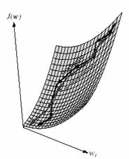
Figure 10.9: The incorporation of momentum into stochastic gradient descent.
Algorithm (Stochastic Backpropagation with Momentum)
begin initialize n H , w , a (<1), q , h , m ¬ 0, bji ¬ 0, bkj ¬ 0
do m ¬ m + 1 (increment epoch)
xm ¬ randomly chosen pattern
bji¬
![]() bkj¬
bkj¬
![]()
wji ¬ wji+ bji ; wkj¬ wkj + bkj
until
![]()
return w
end
One method of simplifying a network and avoiding over-fitting is to impose a heuristic that the weights should be small. There is no principled reason why such a method of “weight decay” should always lead to improved network performance (indeed there are occasional cases where it leads to degraded performance), but it is found in most cases that it helps. The basic approach is to start with a network with “too many” weights and “decay” all weights during training. Small weights favor models that are more nearly linear. One of the reasons weight decay is so popular is its simplicity. After each weight update, every weight is simply “decayed” or shrunk according to
![]() (10.33)
(10.33)
where 0<Î <1. In this way, weights that are not needed for reducing the error function become smaller and smaller, possibly to such a small value that they can be eliminated altogether. Those weights that are needed to solve the problem will not decay indefinitely. In weight decay, then, the system achieves a balance between pattern error and some measure of overall weight. It can be shown that the weight decay is equivalent to gradient descent in a new effective error or criterion function:
![]() (10.34)
(10.34)
The second term on the right-hand side of eq.10.34 is sometimes called a regularization term and in this case preferentially penalizes a single large weight. Another version of weight decay includes a decay parameter that depends upon the value of the weight itself, and this tends to distribute the penalty throughout the network:
 (10.35)
Often we have insufficient training data for the desired classification accuracy and we would like to add information or constraints to improve the network. The approach of learning with hints is to add output units for addressing an assistant problem, one different from but related to the specific classification problem at hand. The expanded network is trained on the classification problem of interest and the assistant one, possibly simultaneously. For instance, suppose we seek to train a network to classify c phonemes based on some acoustic input. In a standard neural network, we would have c output units. In learning with hints, we might add two assistant output units, one which represents vowels and the other consonants. During training, the target vector must be lengthened to include components for the hint outputs. During classification, the hint units are not used; they and their hidden-to-output weights can be discarded (Figure 10.10).
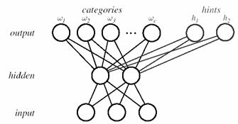
Figure 10.10: Hints added to output units.
The benefit provided by hints is in improved feature selection. So long as the hints are related to the classification problem at hand, the feature groupings useful for the hint task are likely to aid category learning. Learning with hints illustrates another benefit of neural networks: Hints are more easily incorporated into neural networks than into classifiers based on other algorithms, such as the nearest neighbor.
Each of the three leading training protocols has strengths and drawbacks. On-line learning is to be used when the amount of training data is so large, or when memory costs are so high, that storing the data is prohibitive. Most practical neural network classification problems are addressed instead with batch or stochastic protocols. Batch learning is typically slower than stochastic learning. For most applications-especially ones employing large redundant training sets-stochastic training is hence to be preferred. Batch training admits some second-order techniques that cannot be easily incorporated into stochastic learning protocols and hence in some problems should be preferred.
In three-layer networks having many weights, excessive training can lead to poor generalization as the net implements a complex decision boundary “tuned” to the specific training data rather than the general properties of the underlying distributions. In training the two-layer networks, we can usually train as long as we like without fear that it would degrade final recognition accuracy because the complexity of the decision boundary is not changed-it is always simply a hyperplane. For this reason the general phenomenon should be called “overfitting,” not “overtraining.”
Because the network weights are initialized with small values, the units operate in their linear range and the full network implements linear discriminants. As training progresses, the nonlinearities of the units are expressed and the decision boundary warps. Qualitatively speaking, then, stopping the training before gradient descent is complete can help avoid overfitting. In practice, it is hard to know beforehand what stopping criterion q should be set. A far simpler method is to stop training when the error on a separate validation set reaches a minimum. We note in passing that weight decay behaves much like a form of stopped training.
The backpropagation algorithm applies equally well to networks with three, four, or more layers, so long as the units in such layers have differentiable activation functions. Because three layers suffice to implement any arbitrary function, we would need special problem conditions or requirements to recommend the use of more than three layers. Some functions can be implemented more efficiently in networks with more than one hidden layer. It has been found empirically that networks with multiple hidden layers are more prone to getting caught in undesirable local minima, however. In the absence of a problem-specific reason for multiple hidden layers, it is simplest to proceed using just a single hidden layer, but also to try two hidden layer if necessary.
The squared error of eq.10.7 is the most common training criterion because it is simple to compute, is nonnegative, and simplifies the proofs of some theorems. Nevertheless, other training criteria occasionally have benefits. One popular alternative is the cross entropy which measures a “distance” between probability distributions. The cross entropy for n patterns is of the form:
![]() (10.36)
(10.36)
where tmk and zmk are the target and the actual output of unit k for pattern m. Of course, to interpret J as entropy, the target and output values must be interpreted as probabilities and must fall between 0 and 1.
Yet another criterion function is based on the Minkowski error:
![]() (10.37)
(10.37)
It is a straightforward matter to derive the backpropagation rule for this error. While in general the rule is a bit more complex than for the (R = 2) sum-squared error we have considered, the Minkowski error for 1 £ R < 2 reduces the influence of long tails in the distributions-tails that may be quite far from the category decision boundaries. As such, the designer can adjust the “locality” of the classifier indirectly through choice of R; the smaller the R, the more local the classifier.
We have used a second-order analysis of the error in order to determine the optimal learning rate. We can use second-order information more fully in other ways, including the elimination of unneeded weights in a network.
One of the simplest methods for using second-order information to increase training speed is the Quickprop algorithm. In this method, the weights are assumed to be independent, and the descent is optimized separately for each. The error surface is assumed to be quadratic and the coefficients for the particular parabola are determined by two successive evaluations of J(w) and dJ(w)/ dw. The single weight w is then moved to the computed minimum of the parabola (Figure 10.11). It can be shown that this approach leads to the following weight update rule,
 (10.38)
where the derivatives are evaluated at iterations m and m-1, as indicated.
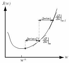
Figure 10. 11: The quickprop weight update takes the error derivatives at two points separated by a known amount, and by computes the next weight value.
If the third- and higher-order terms in the error are non-negligible, or if the assumption of weight independence does not hold, then the computed error minimum will not equal the true minimum, and further weight updates will be needed. When a number of obvious heuristics are imposed-to reduce the effects of estimation error when the surface is nearly flat, or the step actually increases the error-the method can be significantly faster than standard backpropagation. Another benefit is that each weight has, in effect, its own learning rate, and thus weights tend to converge at roughly the same time, thereby reducing problems due to non-uniform learning.
Another fast learning method is conjugate gradient descent, which employs a series of line searches in weight or parameter space. One picks the first descent direction (for instance, the simple gradient) and moves along that direction until the local minimum in error is reached. The second descent direction is then computed: This direction-the conjugate direction-is the one along which the gradient does not change its direction, but merely its magnitude during the next descent. Descent along this direction will not spoil the contribution from the previous descent iterations (Figure 10.12).

Figure 10.12: Conjugate gradient descent in weight space employs a sequence of line searches.
More specifically, we let Dw (m-1) represent the direction of a line search on step m-1. Note especially that this is not an overall magnitude of change, which will be determined by the line search. We demand that the subsequent direction, D w (m), obey
![]() (10.39)
(10.39)
where H is the Hessian matrix. Pairs of descent directions that obey eq.10.39 are called conjugate. If the Hessian is proportional to the identity matrix, then such directions are orthogonal in weight space. Conjugate gradient requires batch training, because the Hessian matrix is defined over the full training set.
The descent direction on iteration m is in the direction of the gradient plus a component along the previous descent direction:
![]() (10.40)
(10.40)
the relative proportions of these contributions is governed by b m. This proportion can be derived by ensuring that, the descent direction on iteration m does not spoil that from direction m-1, and indeed all earlier directions. It is generally calculated in one of two ways. The first formula (Fletcher-Reeves) is
![]() (10.41)
(10.41)
A slightly preferable formula (Polak-Ribiere) that is more robust in nonquadratic error functions is
![]() (10.42)
(10.42)
We now consider an alternative network and training method that have proven effective in special classes of problems. A radial basis function network with linear output units, implements
![]() (10.43)
(10.43)
where we have included a j=0 bias unit. If we define a vector f whose components are the hidden unit outputs, along with a matrix W whose entries are the hidden-to-output weights, then eq.10.43 can be rewritten as z(x) = W f. Minimizing the criterion function
![]() (10.44)
(10.44)
is formally equivalent to the linear problem we saw in Chapter 9. We let T be the matrix consisting of target vectors and let f be the matrix whose columns are the vectors f , then the solution weights obey
![]() (10.45)
(10.45)
and the solution can be written directly:
![]() . Recall that
. Recall that
![]() is the pseudoinverse
of
f.
One of the benefits of such radial basis function or RBF networks
with linear output units is that the solution requires merely such standard
linear techniques. Nevertheless, inverting large matrices can be
computationally expensive, and thus the above method is generally confined to
problems of moderate size.
is the pseudoinverse
of
f.
One of the benefits of such radial basis function or RBF networks
with linear output units is that the solution requires merely such standard
linear techniques. Nevertheless, inverting large matrices can be
computationally expensive, and thus the above method is generally confined to
problems of moderate size.
If the output units are nonlinear, that is, if the network implements
 (10.46)
rather than eq.10.43, then standard backpropagation can be used. One need merely take derivatives of the localized activation functions. For classification problems, it is traditional to use a sigmoid for the output units in order to keep the output values restricted to a fixed range. Some of the computational simplification afforded by sigmoidal activation functions in the hidden units functions is lost, but this presents no conceptual difficulties.
Multiple layers of neurons with nonlinear transfer functions allow the network to learn nonlinear and linear relationships between input and output vectors. It can approximate any function with a finite number of discontinuities, arbitrarily well, given sufficient neurons in the hidden layer. In order to test and simulate the multilayer neural network, the following data is provided as depicted in Figure 10.13.
Figure 10.13: Training pattern used for the simulation of multilayer neural networks.
Neurons may use any differentiable transfer function to generate their output. Multilayer networks often use sigmoid transfer function (logsig). Alternatively, it can use the tangent sigmoid transfer function (tansig). Occasionally, the linear transfer function (purelin) is used in backpropagation networks. If the last layer of a multilayer network has sigmoid neurons, then the output neurons of the network are limited to a small range. If linear output neurons are used the network outputs can take any value. Note that in backpropagation it is important to be able to calculate the derivatives of any transfer function.
The performance of a trained network is measured by the errors on the training, validation and test sets, where it is useful to some extent. However, it is often more explanatory to investigate the network response in more detail. One option is to perform a regression analysis between the network response and the corresponding targets. Thus, the results of the algorithm which is implemented, is given together with the network structure, the validation, test, and training errors plot, and the regression analysis plot.
Matlab script: ccBatchBackpropagation.m (requires ccData1.mat)
(a)
(b) (c)
Figure 10.14: a. Multilayer neural network structure, b. training, validation, test error plot, and c. linear regression analysis.
Number of Neurons in the hidden layer : 2
Epochs : 1000
Learning rate : 0.05
(a)
(b) (c)
Figure 10.15: Multilayer neural network with different parameters. a. Structure. b. training, validation, test error plot, and c. linear regression analysis.
Number of Neurons in the hidden layer : 3
Epochs : 1000
Learning rate : 0.05
(a)
(b) (c)
Figure 10.16: Multilayer neural network with different parameters. a. Structure. b. training, validation, test error plot, and c. linear regression analysis.
Number of Neurons in the hidden layer : 4
Epochs : 1000
Learning rate : 0.05
(a)
(b) (c)
Figure 10.17: Multilayer neural network with different parameters. a. Structure. b. training, validation, test error plot, and c. linear regression analysis.
Number of Neurons in the hidden layer : 3
Epochs : 1000
Learning rate : 0.001
[1] Duda, R.O., Hart, P.E., and Stork D.G., (2001). Pattern Classification. (2nd ed.). New York: Wiley-Interscience Publication.
[2] Neural Network Toolbox For Use With MATLAB, User’s Guide, (2003) Mathworks Inc., ver.4.0
[3] Gutierrez-Osuna R ., Introduction to Pattern Analysis, Course Notes, Department of Computer Science, A&M University, Texas
[4] Sima J. (1998). Introduction to Neural Networks, Technical Report No. V 755, Institute of Computer Science, Academy of Sciences of the Czech Republic
[5] Kröse B., and van der Smagt P. (1996). An Introduction to Neural Networks . (8th ed.) University of Amsterdam Press, University of Amsterdam.
[6] Gurney K. (1997). An Introduction to Neural Networks. (1st ed.) UCL Press, London EC4A 3DE, UK.
[7] Paplinski A.P. Neural Nets. Lecture Notes, Dept. of Computer Sciences, and Software Eng., Manash University, Clayton-AUSTRALIA
[8] Bain J. L, and Engelhardt M. (1991) Introduction to Probability and Mathematical Statistics. (2nd ed.), Duxbury Publication, California-USA