Chapter 2 Matrix Theory and Applications with MATLAB
2.1 Vectors and Matrices
2.1.1 Vector and Matrix Notation>
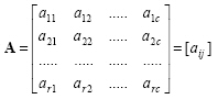
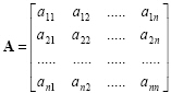
A matrix is a rectangular array, which is arranged as horizontal row and vertical column elements and is shown in brackets. Matrices are shown with bold capital letters. The dimension of a matrix with r rows and c columns is called r by c, and usually written as r x c.
|
(2.1) |
A matrix is called real-valued, if all the elements of the matrix are real valued numbers or functions. If at least one element of a matrix is a complex number or a complex-valued function, the matrix is called complex valued. If all the members of a matrix are numbers, the matrix is refered as a constant matrix.
A matrix with one row or column is called as vector. Vectors are usually shown as a column matrix as:

|
(2.2) |
which are composed of n real elements such that
 . The term
 represents n-dimensional space, and thus, A represents a point in this space. A vector with one row is referred to as row vector, and a vector with one column is referred to as column vector.
2.1.2 Matrices
Matrix Addition, Subtraction, Multiplication
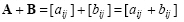
In order to add two matrices, their dimensions should also be equal and is defined as:
|
(2.3) |
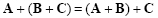
Addition of matrices has associative and commutative properties:
|
(2.4) |

|
(2.5) |
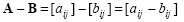
The difference of two matrices is defined similarly as:
|
(2.6) |
The multiplication of a matrix with a scalar value k is obtained by multiplying every element of the matrix with the scalar as:
|
(2.7) |
The elements of matrix C, which is the product of matrix
 with dimension r x p and matrix
 with dimension p x c is calculated as:

|
(2.8) |
Matrix product is associative, distributive over addition and subtraction, but not commutative:
|
(2.9) |
|
(2.10) |
|
(2.11) |

|
(2.12) |
and also

|
(2.13) |
If n is a positive integer and A is a square matrix than the nthpower of A is calculated by multiplying itself n times as

|
(2.14) |
Thus, it is obvious that 
Square matrix, diagonal matrix
A matrix, whose number of rows and columns are equal, is called a square matrix. The general form of a square matrix can be written as
|
(2.15) |
The diagonal elements of this matrix are a11, a22, a33...ann. The matrix whose elements other than the diagonal elements, are zero, is called as a diagonal matrix as:

|
(2.16) |
Identitymatrix
An identity matrix is a diagonal matrix whose diagonal elements is one and represented by I.

|
(2.17) |
The identity matrix has the following property:

|
(2.18) |
Matrix Transpose
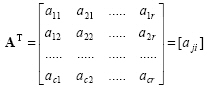
The transpose of a matrix is shown as AT and is simply obtained by writing the rows of A one by one as columns of AT. If the dimension of the matrix A is r x c, the dimension of its transpose is c x r.
|
(2.19) |
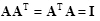
A square matrix is said to be orthonormal if
|
(2.20) |
The rank and trace of a matrix
The rank of a matrix is the number of linearly independent rows (or columns). The trace of a square matrix
 is the sum of its diagonal elements

|
(2.21) |
Matrix inverse
The inverse of a matrix  is depicted by
 and defined such that

|
(2.22) |
The inverse of a matrix
exists if and only if A is non-singular.
Singular matrix
A matrix is said to be singular if its inverse does not exist, otherwise non-singular. The rank of a non-singular matrix equals the number of rows (or columns).A non-singular matrix has a non-zero determinant. If A is non-singular, than

|
(2.23) |
Two non-singular matrices A and B are:

|
(2.24) |
If A is non-singular than  is also non-singular and

|
(2.25) |
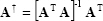
Pseudo-inverse matrix
The pseudo-inverse matrix
 is typically used whenever
does not exist (because A is not square or A is singular):
is typically used whenever
does not exist (because A is not square or A is singular):
|
(2.26) |
assuming that  and
and
 is non-singular. Also in general it can be stated that
  .
.
Determinant
The determinant of a square matrix is represented as det A, or as |A|, and is a scalar value and calculated for 2 × 2 matrices as:
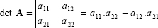
|
(2.27) |
For n>2, the determinant of n × n matrices is calculated by reducing the matrix and using minors as follows. The minor Mij of a matrix An×n is the determinant of n-1 × n-1 sub-matrix which is formed by removing the ith row and jth column from A. Thus the determinant of A has the form:
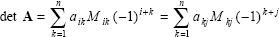
|
(2.28) |
Here is an example:
The determinant of 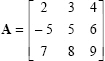 can be opened through first row or first column such as
or
Some properties of determinants can be states as follows. For two square matrices An×n and Bn×n which are equally dimensioned
|
(2.29) |
For a square matrix An×n

|
(2.30) |
If the inverse of A exists than
|
(2.31) |
Eigen-vectors and eigen-values
For a square matrix An×n and a column vector X, if there exists a scalar value such that

|
(2.32) |
the vector X is called the eigen-vector of matrix A, and scalar is called the corresponding eigen-value. Here is an example:
For

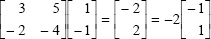 can be provided. Therefore, the vector
  , is the eigen-vector, corresponding to eigen-value
  ,
of A.
,
of A.
Eigen values can be computed as follows:

|
(2.33) |
For the non-trivial solution:
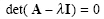
|
(2.34) |
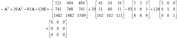
Cayley-Hamilton theorem states that each square matrix provides its own eigen-equation (characterisic equation) such that if

|
(2.35) |
than

|
(2.36) |
Follow the example
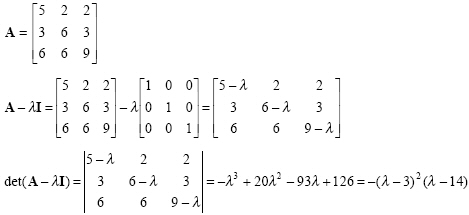
which is the characterisic equation. Thus, it can be shown that matrix A provides Cayley-Hamilton theorem
Eigen-values and eigen-vectors have the following properties. If A is non-singular, all eigen-values of A are non-zero. If A is real and symmetric, all eigrn-values are real and the eigen-vectors associated with distinct eigen-values are orthogonal. If A is positive definite, than all the eigen-values are positive. In addition, the eigen-values of a matrix and its transpose are equal.
2.1.3 Vectors
Magnitude (norm)
The magnitude (Euclidean norm) of any vector is represented by and given as
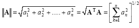
|
(2.37) |
Inner product (dot product)
The inner product (dot product) of two vectors A and B, with equal dimensions, is calculated by mutually multiplying the elements, and then by adding as:
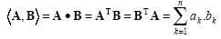
|
(2.38) |
and the result is a scalar.
The inner product given in eq. 2.38 can also be calculated as
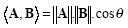
|
(2.39) |
where is the angle between two vectors.
Orthogonal and orthonormal vectors
Two vectors A and B are said to be orthogonal if their inner product is equal to zero:

|
(2.40) |
and two vectors are said to be orthonormal if they are orthogonal and each of them are unit vectors such that:
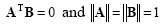
|
(2.41) |
Projection
The orthogonal (parallel) projection of vector A onto vector B is shown in Figure 2.1 and calculated as
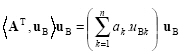
|
(2.42) |
where is a unit vector such that and is in the same direction with .
Figure 2.1: The projection of vector A onto vector B.
2.1.4 Linear Transformations
A common linear equation system is a group of equations such that :
|
|
(2.43) |
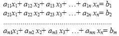
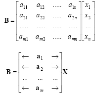
The coefficients aij (i=1,2,...,m; j=1,2,...,n) and bi (i=1,2,...,m) are known scalars, and xj (j=1,2,...,m) are unknown variables. This system is equavalent of the following matrix system:

|
(2.44) |
where
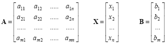
The matrix A is called coefficients-matrix since it includes all the coefficients of the system. The ith row (i=1,2...m) of A corresponds to the ith equation of system given in eq.2.43. Notice that the dimensionality of the two spaces does not need to be the same. For pattern recognition we typically have m < n which means that we project onto a lower-dimensionality space.
Linearly dependent / independent vectors
A n-dimensional set of vectors whose individual elements are in equal dimensions, {V1, V2, …, Vn}are said to be linearly dependent if there exists a set of coefficients a1, a2, …, an (at least one different than zero) which provides
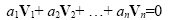
|
(2.45) |
Alternatively, a set of vectors V1, V2, …, Vn are said to be linearly independent if

|
(2.46) |
Linear orthonormal transformation
A linear transformation represented by a square matrix A is said to be orthonormal when

|
(2.47) |
which implies that

|
(2.48) |
An orthonormal matrix can be thought of as a rotation of the reference frame. An orthonormal transformation has the property of preserving the magnitude of the vectors as:

|
(2.49) |
The row vectors of an orthonormal transformation form a set of orthonormal basis vectors:
|
(2.50) |
2.1.5 Vector Spaces
The n-dimensional space in which all the n-dimensional vectors reside is called a vector space. A set of vectors {u1, u2, ... un} is said to form a basis for a vector space if any arbitrary vector V can be represented by a linear combination of the {u1, u2, ... un}.
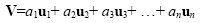
|
(2.51) |
The coefficients {a1, a2, ... an} are called the components of vector V with respect to the basis vectors {u1, u2, ... un}. In order to form a basis, it is necessary and sufficient that the basis vectors {u1, u2, ... un} be linearly independent.
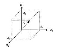 Figure 2.2: Representation of a vector using basis vectors and coefficients in vector space. |
Orthogonal and orthonormal vector sets
A set of vectors such as basis vectors {u1, u2, ... un} is said to orthogonal if each of the vectors within the set are orthogonal to each of the remaining vectors within the set. That is:
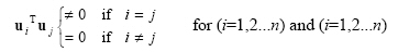
|
(2.52) |
where n is number of vectors in the set. Such a set is linearly independent if all the vectors are non- zero.
A set of vectors such as basis vectors {u1, u2, ... un} is said to orthonormal if the set is orthogonal and all of the vectors within the vectors are unit vectors.
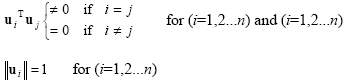
|
(2.53) |
Thus
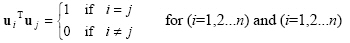
|
(2.54) |
The 2D and 3D Cartesian coordinate systems are orthonormal, as their basis vectors orthogonal and each of them are unit vectors.
Gram-Schmidt orthonormalization procedure
Related with every finite linearly independent set of vectors such as {X1, X2, ... Xn}, an orthogonal set of vectors {Q1, Q2, ... Qn}whose individual elements are non-zero, exists, such that each vector Qj (j=1,2...n), is a linear combination of vectors X1 through X j-1. The algorithm that composes Qj vectors is known as Gram-Schmidt orthogonalization procedure. Since this method is very sensitive to rounding errors, it can generate wrong results under finite digit arithmetics. A uniform variation of Gram-Schmidt orthogonalization procedure can generate the same vectors when rounding does not applied. The second method is recursive and transforms the linearly independent set of vectors {X1, X2, ... Xn} into orthonormal set of vectors {Q1, Q2, ... Qn} such that every Qj (j=1,2...n), is a linear combination of vectors X1 through X j-1. The kth recurrence of the algorithm is as follows:
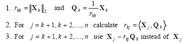
|
(2.55) |
Euclidean distance
The distance between two points in a vector space is defined as the magnitude of the vector difference between the points (Figure 2.3). That is
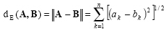
|
(2.56) |
This distance is known as Euclidean distance.
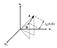 Figure 2.3: Euclidean distance between two vectors.
|
2.2 Matrix Operations in MATLAB
The transition from mathematics to code or vice versa can be made with the aid of a few rules in MATLAB. It will be useful to list them here for future reference. To change from mathematics notation to MATLAB notation, the user needs to:
•Change superscripts to cell array indices:

•Change subscripts to parentheses indices:  )
)
•Change parentheses indices to a second cell array index: 
•Change mathematics operators to MATLAB operators and toolbox functions: 
2.2.1 Array Construction
In MATLAB, a matrix is a rectangular array of numbers. When they are taken away from the world of linear algebra, matrices become two-dimensional numeric arrays.
Manuel construction
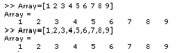
Arrays are constructed by declaring its elements within brackets “[]” separating each element with a space or a comma.
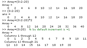
The 1:n shorthand
An array can simply be constructed by using colon operator“:”. The syntax fro this command is as (begining value : increment : ending value). Here are examples of its variations.
The linspace command
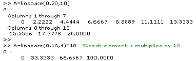
The linspace command generates linearly spaced vectors. It is similar to the colon operator ":", but gives direct control over the number of points. The syntax is as
y = linspace(a,b) generates a row vector y of 100 points linearly spaced between and including a and b.
y = linspace(a,b,n) generates a row vector y of n points linearly spaced between and including a and b.
Generally its syntax can be rewritten as:
linspace(beginning value, ending value, number of elements to be generated)
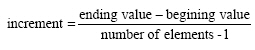
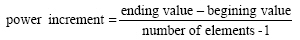
The spacing between elements of the array generated by the linspace command is calculated as:
The logspace command
The logspace command generates logarithmically spaced vectors. It is especially useful for creating frequency vectors, it is a logarithmic equivalent of linspace and the colon operator ":". All the arguments to logspace command must be scalars. The syntax is as
y = logspace(a,b) generates a row vector y of 50 logarithmically spaced points between decades  and
and
 10b.
10b.
y = logspace(a,b,n) generates n points between decades
and
.
y = logspace(a,pi) generates the points between
and
 ,
which is useful for digital signal processing where frequencies over this interval go around the unit circle.
,
which is useful for digital signal processing where frequencies over this interval go around the unit circle.
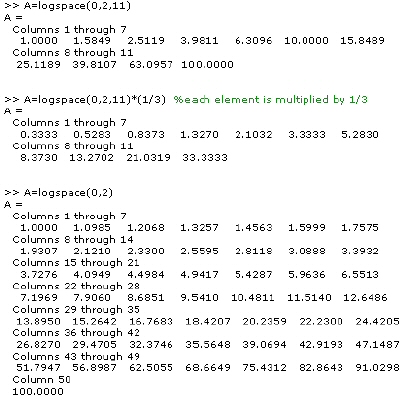
Generally its syntax can be rewritten similar to linspace command as:

The spacing between elements of the array generated by the logspace command is calculated as:
2.2.2 Matrix Construction
Manuel construction
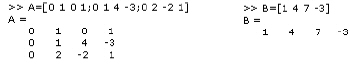
In MATLAB, a matrix is a rectangular array of numbers. When they are taken away from the world of linear algebra, matrices become two-dimensional numeric arrays. The semicolon operator “;”, when used inside brackets, ends rows. Thus, an array (vector or matrix) can be created using semicolon operator as follows:
A matrix and a row vector is defined as:
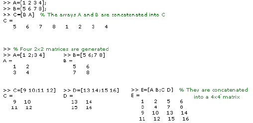
Concatenating arrays and matrices
Concatenation is the process of joining small arrays/matrices to make bigger ones. In fact, we made our first matrix by concatenating its individual elements. The pair of square brackets, [], is the concatenation operator.
2.2.3 Array and Matrix Indexing
The colon operator “:” is used for creating vectors, and array subscripting and it uses the rules given in Table 2.1 to create regularly spaced vectors.
Table 2.1: The rules for colon operator.
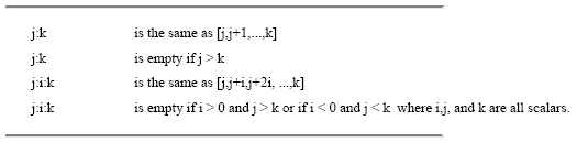
Table 2.2 gives the definitions that govern the use of the colon to pick out selected rows, columns, and elements of vectors, matrices, and higher-dimensional arrays.
Table 2.2: The definitions for governing the colon operator “ : ”.

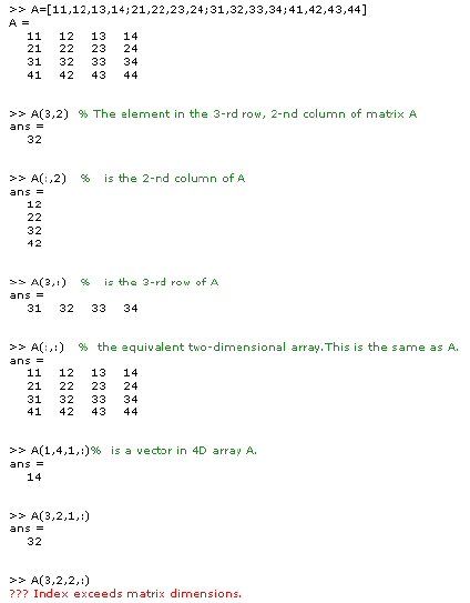
The examples of the definitions given in Table 2.2 are as follows.
2.2.4 Array and Matrix Operations
Arithmetic operations on arrays are done element-by-element. This means that addition and subtraction are the same for arrays and matrices, but that multiplicative operations are different.
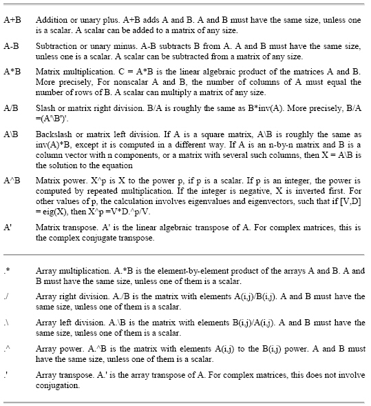
The matrix operations discussed above can be implemented with MATLAB. The operators for matrix and array manipulation of MATLAB are given in Table 2.3. Their usage and basic operations in MATLAB will be examined with source code below.
Table 2.3: Matrix operators used in MATLAB. .
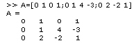
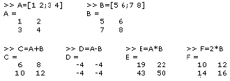
A matrix is defined as:
A vector and its transpose:
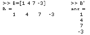
Basic matrix operations:
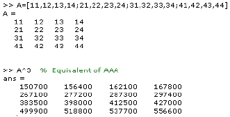
The power of a matrix is calculated as:
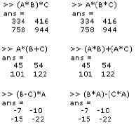
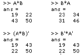
Implementations of equations 2.9 through 2.13 are depicted below.
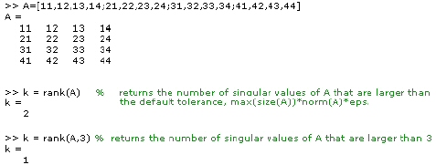
The rank function
The rank function provides an estimate of the number of linearly independent rows or columns of a matrix. There are a number of ways to compute the rank of a matrix. MATLAB uses the method based on the singular value decomposition (SVD). The SVD algorithm is the most time consuming, but also the most reliable.
k = rank(A) returns the number of singular values of A that are larger than the default tolerance, max(size(A))*norm(A)*eps.
k = rank(A,tol) returns the number of singular values of A that are larger than tol.
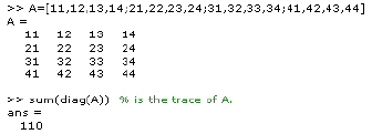
The diag function
The trace of a matrix, given by eq. 2.21, is not provided directly. It is calculated as a combination of functions diag and sum as
sum(diag(X)) is the trace of X.
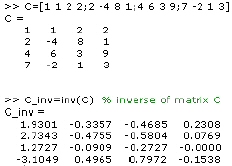
The inv function
The inverse of A, is denoted by A-1, and is computed by the function inv as follows.
The det function and singular matrix
The determinant of a matrix is computed by the function det as follows.
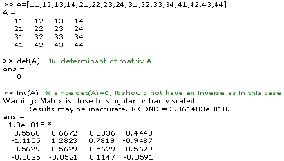
If the determinant of a particular matrix happens to be zero, it indicates that the matrix is singular. Since the matrix is singular, it does not have an inverse. When we tried to compute the inverse we got a warning message.
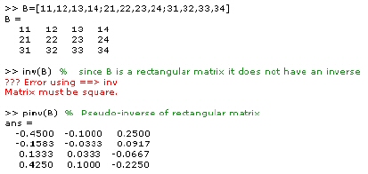
The pinv function
Since rectangular matrices do not have inverses or determinants the pseudoinverse of a matrix is computed using the function pinv as follows.
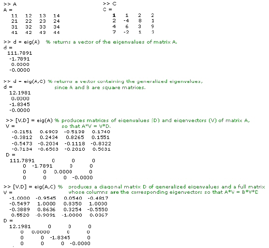
The eig function
The eigen-values and eigen-vectors are computed using the eig function as follows.
d = eig(A) returns a vector of the eigenvalues of matrix A.
d = eig(A,B) returns a vector containing the generalized eigenvalues, if A and B are square matrices.
[V,D] = eig(A) produces matrices of eigenvalues (D) and eigenvectors (V) of matrix A, so that A*V = V*D. Matrix D is the canonical form of A - a diagonal matrix with A's eigenvalues on the main diagonal. Matrix V is the modal matrix--its columns are the eigenvectors of A. For eig(A), the eigenvectors are scaled so that the norm of each is 1.0. Use [W,D] = eig(A.'); W = W.' to compute the left eigenvectors, which satisfy W*A = D*W.
[V,D] = eig(A,B) produces a diagonal matrix D of generalized eigenvalues and a full matrix V whose columns are the corresponding eigenvectors so that A*V = B*V*D.
[V,D] = eig(A,B,flag) specifies the algorithm used to compute eigenvalues and eigenvectors. Flag can be: ‘chol’ Computes the generalized eigenvalues of A and B using the Cholesky factorization of B. This is the default for symmetric (Hermitian) A and symmetric (Hermitian) positive definite B. ‘qz’ ignores the symmetry, if any, and uses the QZ algorithm as it would for nonsymmetric (non-Hermitian) A and B.
The eigenvalue problem is to determine the nontrivial solutions of the equation where A is an n-by-n matrix, x is a length n column vector, and is a scalar. The n values of that satisfy the equation are the eigenvalues, and the corresponding values of x are the right eigenvectors. In MATLAB, the function eig solves for the eigenvalues, and optionally the eigenvectors x. The generalized eigenvalue problem is to determine the nontrivial solutions of the equation where both A and B are n-by-n matrices and is a scalar. The values of that satisfy the equation are the generalized eigenvalues and the corresponding values of x are the generalized right eigenvectors. If B is nonsingular, the problem could be solved by reducing it to a standard eigenvalue problem. Because B can be singular, an alternative algorithm, called the QZ method, is necessary. When a matrix has no repeated eigenvalues, the eigenvectors are always independent and the eigenvector matrix V diagonalizes the original matrix A if applied as a similarity transformation. However, if a matrix has repeated eigenvalues, it is not similar to a diagonal matrix unless it has a full (independent) set of eigenvectors. If the eigenvectors are not independent then the original matrix is said to be defective. Even if a matrix is defective, the solution from eig satisfies A*X = X*D.:
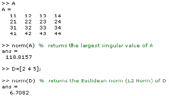
The norm function
The norm of a matrix is a scalar that gives some measure of the magnitude of the elements of the matrix. The norm function calculates several different types of matrix norms. The one which we deal with is as follows.
n = norm(A) returns the largest singular value of A, max(svd(A))
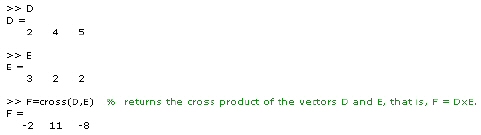
The cross function
The cross product is computed using the function dot as follows.
C = cross(A,B) returns the cross product of the vectors A and B. That is, C = A B. A and B must be 3-element vectors. If A and B are multidimensional arrays, cross returns the cross product of A and B along the first dimension of length 3.
C = cross(A,B,dim) where A and B are multidimensional arrays, returns the cross product of A and B in dimension dim . A and B must have the same size, and both size(A,dim) and size(B,dim) must be 3.
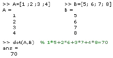
The dot function
The dot product is computed using the function dot as follows.
2.2.5 Standard Arrays and Matrices
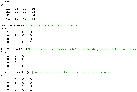
The eye function
The eye function is used to generate an Identity matrix as follows.
Y = eye(n) returns the n-by-n identity matrix.
Y = eye(m,n) or eye([m n]) returns an m-by-n matrix with 1's on the diagonal and 0's elsewhere.
Y = eye(size(A)) returns an identity matrix the same size as A
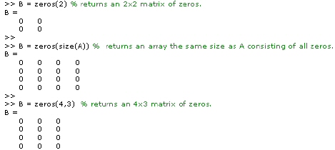
The ones and zeros functions
The zeros function creates an array of all zeros as follows.
B = zeros(n) returns an n-by-n matrix of zeros. An error message appears if n is not a scalar.
B = zeros(size(A)) returns an array the same size as A consisting of all zeros.
B = zeros(m,n) or B = zeros([m n]) returns an m-by-n matrix of zeros.
B = zeros(d1,d2,d3...) or B = zeros([d1 d2 d3...]) returns an array of zeros with dimensions d1-by-d2-by-d3-by-... .
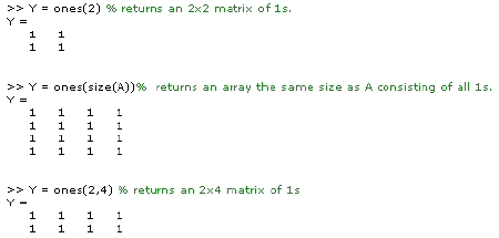
The ones function creates an array of all ones as follows.
Y = ones(n) returns an n-by-n matrix of 1s. An error message appears if n is not a scalar.
Y = ones(size(A)) returns an array the same size as A consisting of all 1s.
Y = ones(m,n) or Y = ones([m n]) returns an m-by-n matrix of 1s.
Y = ones(d1,d2,d3...) or Y = ones([d1 d2 d3...]) returns an array of 1s with dimensions d1-by-d2-by-d3-by-... .
2.2.6 Array and Matrix Size
The size function
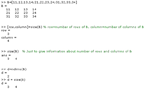
The size of an array or matrix can be learned by using the size function such that:
d = size(X) returns the sizes of each dimension of array X in a vector d with ndims(X) elements.
[r,c] = size(X) returns the size of matrix X in variables r and c.
m = size(X,dim) returns the size of the dimension of X specified by scalar dim.
[d1,d2,d3,...,dn] = size(X) returns the sizes of the various dimensions of array X in separate variables.
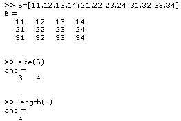
The length function
The statement length(X) returns the longest dimension of the matrix defined by its parameter, and is equivalent to max(size(X)) for nonempty arrays and 0 for empty arrays. If X is a vector, the returned value is the same as its length.
REFERENCES
[1] Bronson R., (1989) Matrix Operations Theory, and Practice, Schaum’s Outline Series, McGraw-Hill Companies Inc.
[2] Adams R. A., (2003) Calculus: A Complete Course, (5th Ed.), Toronto: Pearson Education, Canada.
[3] Gutierrez-Osuna R., Introduction to Pattern Analysis, Course Notes, Department of Computer Science, A&M University, (http://research.cs.tamu.edu/prism/lectures/pr/pr_l1.pdf ), Texas
[4] Arifoğlu, U., and Kubat C., (2003). MATLAB ve Mühendislik Uygulamaları.İstanbul: ALFA Basım Yayım Dağıtım Ltd. Şti.
[5] Demuth H., and Beale M. (2003). Neural Network Toolbox For Use With MATLAB, User’s Guide, Mathworks Inc., version 4.0