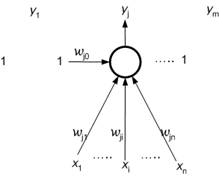
The first successful model of neural network in the history of neurocomputing was the network of perceptrons. The architectural dynamics of this network specifies a fixed architecture of a one-layered network n-m at the beginning. This means that the network consists of n input neurons, each being an input for all m output neurons as it is depicted in Figure 8.1. Denote by x1… xn the real states of input neurons, x=(x1…xn) Î Rn is the network input, and denote by y1… ym the binary states of output neurons, y=(y1…ym) Î {0, l}m is the network output. Furthermore, wij represents a real synaptic weight associated with the connection leading from the ith input neuron (i=1,.., n) to the jth output neuron (j=1, ... , m), and wj0 =-h j is a bias (a threshold hj with the opposite sign) of the jth output neuron corresponding to a formal unit input x0=1.
Figure 8.1 : The architecture of the Network of Perceptrons.
The computational dynamics of the network of perceptrons determines how the network function is computed. In this case, the real states of neurons in the input layer are assigned to the network input and the output neurons compute their binary states determining the network output in the same way as the formal neuron does (see eq.7.3)). This means that every perceptron computes its excitation level first as the corresponding affine combination of inputs:
![]() where
where
![]() (8.1)
(8.1)
The coefficients w=(w10,…,w1n,…,wm0,…,wmn) create the network configuration. Then the perceptron state is determined from its excitation level by applying an activation function
s : R ® {0,1} (8.2)
such as the hard limiter. This means, that the function
y (w) : R ® {0,1}m (8.3)
of the network of perceptrons, which depends on the configuration w, is given by the following equation:
![]()
![]() where
where
![]() (8.4)
(8.4)
A single perceptron can be used to classify input patterns into two classes. This classification is characterized in terms of hyperplanes splitting up the input data space. A linear combination of weights for which the augmented activation potential (excitation level with bias included) is zero, describes a decision surface which partitions the input space into two regions. The decision surface is a hyperplane specified as:
w.x=0, x0=1
or
![]() (8.5)
(8.5)
The weighted sum (including bias term) of a hidden unit clearly defines an n-1 dimensional hyperplane in n-dimensional space. These hyperplanes are seen as decision boundaries, many of which together can carve out complex regions necessary for classification of complex data.
Figure 8.2 : Geometrical interpretation of a neuron function.
The geometrical interpretation depicted in Figure 8.2 may help its to better understand the function of a single neuron. The n input values of a neuron may be interpreted as coordinates of a point in the n-dimensional Euclidean input space. In this space, the equation of a hyperplane has the following form:
![]() (8.6)
(8.6)
This hyperplane disjoins the input space into two halfspaces. The
coordinates
![]() of points that are
situated in one halfspace, meet the following inequality:
of points that are
situated in one halfspace, meet the following inequality:
![]() (8.7)
(8.7)
The points
![]() from the second,
remaining halfspace fulfill the dual inequality with the opposite relation
symbol:
from the second,
remaining halfspace fulfill the dual inequality with the opposite relation
symbol:
![]() (8.8)
(8.8)
Hence, the synaptic weights w0,...,w1 (including bias) of a neuron may be understood as coefficients of this hyperplane. Clearly, such a neuron classifies the points in the input space (the coordinates of these points represent the neuron inputs) to which from two halfspaces determined by the hyperplane they belong, the neuron realizes the dichotomy of input space. More exactly, the neuron is active (the neuron state is y=1) if its inputs meet eq. 8.7 or eq. 8.8, they represent the coordinates of a point that lies in the first halfspace or on the hyperplane. In the case that this point is located in the second halfspace, the inputs of neuron fulfill the eq. 8.9 and the neuron is passive (the neuron state is y=0). The input patterns that can be classified by a single perceptron into two distinct classes are called linearly separable patterns.
In order to generalise to higher dimensions, and to relate vectors to the ideas of pattern space, it is convenient to describe vectors with respect to a cartesian coordinate system. That is, we give the projected lengths of the vector onto two perpendicular axes (see Figure 8.3).
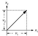
Figure 8.3 : Vector depicted in cartesian axes.
The vector is now described by the pair of numbers ( v1, v2 ). These numbers are its components in the chosen coordinate system. Since they completely determine the vector, we may think of the vector itself as a pair of component values and write v=( v1, v2 ). The vector is now an ordered list of numbers. Notice the ordering is important, since (1,3) is in a different direction from (3,1). This definition immediately generalises to more than 2-dimensions. An n-dimensional vector is simply an ordered list of n numbers, v=(v1 , v 2,...vn). The weight vector w=(w1 , w 2,... , wn) and the input vector x=(x1, x2…xn) are depicted similarly.
For our 2-D prototype, the length of a vector is just its length in the plane. In terms of its components, this is given by Pythagoras’s theorem.
![]() (8.9)
(8.9)
In n-dimensions, the length is defined by the natural extension of eq.8.9
![]() (8.10)
(8.10)
Consider the vectors v=(1, 1) and w=(0, 2) shown below:
Figure 8.4 : Two vectors at 45o.
The angle between them is 45o. Define the inner product v.w of the two vectors by
![]() (8.11)
(8.11)
The form on the right-hand side should be familiar; it is just the same as that, we have used to define the activation of a perceptron. Substituting the component values gives v.w=2. We will now try to give this a geometric interpretation.
First we note that
![]() and
and
![]() . Next, we observe
that the cosine of the angle between the vectors is
. Next, we observe
that the cosine of the angle between the vectors is
![]() .
.
Figure 8.5 : Diagram of cos 45.
Therefore
![]() . It may be shown that this
is a general result; that is, if the angle between two vectors v and w
is
. It may be shown that this
is a general result; that is, if the angle between two vectors v and w
is
![]() then the definition of dot product given in eq.8.11 is equivalent to
then the definition of dot product given in eq.8.11 is equivalent to
![]() (8.12)
(8.12)
In n-dimensions the inner product is defined by the natural extension of eq. 8.11
![]() (8.13)
(8.13)
Although, we cannot now draw the vectors (for n > 3) the geometric insight we obtained for 2-D may be carried over since the behaviour must be the same (the definition is the same). We therefore now examine the significance of the inner product in two dimensions. Essentially the inner product tells us how well ‘aligned’ two vectors are. To see this, let vw be the component of v along the direction of w, or the projection of v along w.
Figure 8.6 : Vector projection.
The projection is given by
![]() which, by eq.
8.12 gives us
which, by eq.
8.12 gives us ![]()
If
![]() is
small then
is
small then ![]() is
close to its maximal value of one. The inner product, and hence the projection
vw,
will be close to its maximal value; the vectors ‘line up’ quite
well. If
is
close to its maximal value of one. The inner product, and hence the projection
vw,
will be close to its maximal value; the vectors ‘line up’ quite
well. If
![]() =90°
, the cosine term is zero and so too is the inner product. The
projection is zero because the vectors are at right angles; they are said to be
orthogonal. If 90 <
=90°
, the cosine term is zero and so too is the inner product. The
projection is zero because the vectors are at right angles; they are said to be
orthogonal. If 90 <
![]() <
270, the cosine is negative and so too, therefore, is the
projection; its magnitude may be large but the negative sign indicates that the
two vectors point into opposite half-planes.
<
270, the cosine is negative and so too, therefore, is the
projection; its magnitude may be large but the negative sign indicates that the
two vectors point into opposite half-planes.
Using the ideas developed above we may express the action of a perceptron in terms of the weight and input vectors. The activation potential may now be expressed as
![]() (8.14)
(8.14)
The vector equivalent to
![]() now becomes
now becomes
![]() (8.15)
(8.15)
If w and w 0 x 0 are constant then this implies the projection xw, of x along w is constant since
![]() (8.16)
(8.16)
In 2-D, therefore, the equation specifies all x which lie on a line perpendicular to w.
Figure 8.7 : w.x= constant
There are now two cases
1. If
![]() , then x must lie beyond the
dotted line
, then x must lie beyond the
dotted line
Figure 8.8 : w.x > w0x0
Using ![]() we
have that
we
have that ![]() implies
implies
![]() that
is, the activation potential is greater than the threshold
that
is, the activation potential is greater than the threshold
2.
Conversely, if
![]() then x must lie below the
dotted line
then x must lie below the
dotted line
 OR
OR 
Figure 8.9 : w.x < w0x0
Using ![]() we
have that
we
have that ![]() implies
implies
![]() ; that
is, the activation potential is less than the threshold
; that
is, the activation potential is less than the threshold
In 3-D the line becomes a plane intersecting the cube and in n-D a hyperplane intersecting the n-dimensional hypercube or n-cube.
Note that the weight vector, w, is orthogonal to the decision plane in the augmented input space because
w.x = 0 (8.17)
that is inner product of the weight and the augmented input vectors is zero. Note that the weight vector is also orthogonal to the decision plane
w.x + w0 x0 = 0 (8.18)
in the proper, (n-1) dimensional input space, where w=(w 1 , w 2 ,... , wn) and x=(x 1 , x 2 …x n ).
In order for the perceptron to perform a desired task, its weights must be properly selected. In general, two basic methods can be employed to select a suitable weight vector.
· By off-line calculation of weights: if the problem is relatively simple, it is often possible to calculate the weight vector from the specification of the problem.
· By learning procedure: the weight vector is determined from a given (training) set of input-output vectors (exemplars) in such a way to achieve the best classification of the training vectors.
Once the weights are selected, the perceptron performs its desired task.
Consider the problem of building a AND gate using the perceptron. In this case, the desired input-output relation is specified by the truth table and related plot given in Figure 8.10.
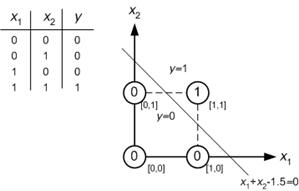
Figure 8.10 : The truth table of AND gate and its implementation.
The input patterns (vectors) belong to two classes and are marked in the input space. The decision plane is the straight line described by te following equation:
x 1 + x 2 -1.5=0 (8.19)
In order for the weight vector to point in the direction of y=1 patterns we select it as w=[1 1 -1.5] For each input vector the output signal is now calculated as
 ;
;
![]() (8.20)
(8.20)
The single perceptron network is depicted in Figure 8.11.
Figure 8.11 : Single perceptron network of AND gate.
Learning is a recursive procedure of modifying weights from a given set of input-output patterns. For a single perceptron, the objective of the learning procedure is to find a decision plane, which separates two classes of given input-output training vectors. Once the learning is finalised, every input vector will be classified into an appropriate class. A single perceptron can classify only the linearly separable patterns. The perceptron learning procedure is an example of a supervised error-correcting learning law.
In an adaptive mode the desired function of the network of perceptrons is given by a training set:
 (8.21)
where xk is a real input of the kth training pattern, and dk is the corresponding desired binary output (given by a teacher). The aim of adaptation is to find a configuration w such that for every input x k (k=1,...,p) from training set T, the network responds with the desired output dk in computational mode, it holds:
y (w, xk) = dk k=1,...,p , and w=(w10,…,w1n,…,wm0,…,wmn) (8.22)
We can assume that an untrained perceptron can generate an incorrect output y ¹d k due to incorrect values of weights. We can think about the actual output y as an estimate of the correct, desired output dk.
The perceptron learning law also known as the perceptron convergence procedure can be described as follows.
1. At the beginning of adaptation, at time 0, the weights of configuration w (0) are initialized randomly close to zero,
![]() ,
where
,
where ![]() ,
and (
j=1,...,m, i=0,...,n ). (8.23)
,
and (
j=1,...,m, i=0,...,n ). (8.23)
2. The network of perceptrons has discrete adaptive dynamics. At each adaptation time step t=1, 2, 3,... one pattern from the training set is presented to the network which attempts to learn it. The actual output yj, is compared with the desired output, dkj, and the error ekj is calculated as
![]() (8.24)
(8.24)
![]() ,
or
,
or
![]() (8.25)
(8.25)
Note that
![]() ,
then
,
then ![]() (8.26)
(8.26)
3. At each step, the weights are adapted as follows
![]() (8.27)
(8.27)
where 0<
![]() <1 is the learning rate (gain),
which controls the adaptation rate. Since we do not want to make too drastic a
change as this might upset previous learning, we add a fraction to weight
vector to produce a new weight vector. The gain must be adjusted to ensure the
convergence of the algorithm. The total expression can be rewritten as
<1 is the learning rate (gain),
which controls the adaptation rate. Since we do not want to make too drastic a
change as this might upset previous learning, we add a fraction to weight
vector to produce a new weight vector. The gain must be adjusted to ensure the
convergence of the algorithm. The total expression can be rewritten as
![]() (8.28)
(8.28)
The expression
![]() in eq.8.28 is
the discrepancy between the actual jth network output for the
kth pattern input and the corresponding desired output of
this pattern. Hence, this determines the error of the jth
network output with respect to the kth training pattern.
Clearly, if this error is zero, the underlying weights are not modified.
Otherwise, this error may be either 1 or -1 since only the binary outputs are
considered. The inventor of the perceptron, Rosenblatt showed that the adaptive
dynamics eq.8.28 guarantees that the network finds its configuration (providing
that it exists) in the adaptive mode after a finite number of steps, for which
it classifies all training patterns correctly (the network error with respect
to the training set is zero), and thus the condition eq.8.22 is met.
in eq.8.28 is
the discrepancy between the actual jth network output for the
kth pattern input and the corresponding desired output of
this pattern. Hence, this determines the error of the jth
network output with respect to the kth training pattern.
Clearly, if this error is zero, the underlying weights are not modified.
Otherwise, this error may be either 1 or -1 since only the binary outputs are
considered. The inventor of the perceptron, Rosenblatt showed that the adaptive
dynamics eq.8.28 guarantees that the network finds its configuration (providing
that it exists) in the adaptive mode after a finite number of steps, for which
it classifies all training patterns correctly (the network error with respect
to the training set is zero), and thus the condition eq.8.22 is met.
The order of patterns during the learning process is prescribed by the so-called training strattegy and it can be, for example, arranged on the analogy of human learning. One student reads through a textbook several times to prepare for an examination, another one learns everything properly during the first reading, and as the case may be, at the end both revise the parts which are not correctly answered by them. Usually, the adaptation of the network of perceptrons is performed in the so-called training epoch in which all patterns from the training set are systematically presented (some of them even several times over). For example, at time t = (c-l) p + k (where 1 £ k £ p) corresponding to the cth training epoch the network learns the kth training pattern.
Considering the network of perceptrons is capable of computing only a restricted class of functions, the significance of this model is rather theoretical. In addition, the above-outlined convergence theorem for the adaptive mode does not guarantee the learning efficiency, which has been confirmed by time-consuming experiments. The generalization capability of this model is also not revolutionary because the network of perceptrons can only be used in cases when the classified objects are separable by hyperplanes in the input space (special tasks in pattern recognition, etc.). However, this simple model is a basis of more complex paradigms like a general feedforward network with the backpropagation-learning algorithm.
In a modified version of the perceptron learning rule,
in addition to misclassification, the input vector x must be located far
enough from the decision surface, or, alternatively, the net activation
potential (augmented)
![]() must exceed a preset margin,
must exceed a preset margin,
![]() . The reason for
adding such a condition is to avoid an erroneous classification decision in a
situation when
. The reason for
adding such a condition is to avoid an erroneous classification decision in a
situation when ![]() is
very small, and due to presence of noise, the sign of
is
very small, and due to presence of noise, the sign of
![]() cannot be reliably
established.
cannot be reliably
established.
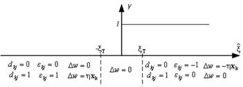
Figure 8.12 : Tabular and graphical illustration of perceptron learning rule.
Using the perceptron training algorithm, we may use a perceptron to classify two linearly separable classes A and B. Examples from these classes may have been obtained, for example, by capturing images in a framestore; there may have been two classes of faces, or we want to separate handwritten characters into numerals and letters.
Figure 8.13 : A / B classification.
The network can now be used for calssification task: it can decide whether an input pattern belongs to one of two classes. If the total input is positive, the pattern will be assigned to class +1, if the total input is negative, the sample will be assigned to class –1. The separation between the two classes in this case is a straight line given by the equation:
![]() (8.29)
(8.29)
where q denotes threshold. The single layer network represents a linear discriminant function. A geometrical representation of the linear threshold neural network is given in eq.8.29 can be written as
![]() (8.30)
(8.30)
and we see that the weights determine the slope of the line and the bias determines the offset, i.e. how far the line is from the origin. Note that also weights can be plotted in the input space: the weight vector is always perpendicular to the discriminant function.
Figure 8.14 : Geometric representation of the discriminant function and the weights.
Suppose now there is four classes A, B, C, D, and that they are separable by two planes in pattern space.
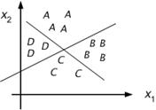
Figure 8.15 : Pattern space for A, B, C, and D.
That is the two classes (A, B) (C, D) are linearly separable, as too are the classes (A, D) and (B, C). We may now train two units to perform these two classifications. Figure 8.16 gives a table encoding the original 4 classes.
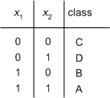
Figure 8.16 : Input coding for A, B, C, and D.
One neuron can solve only very simple tasks. The exclusive disjunction XOR is a typical example of a logical function that cannot be implemented by one neuron. For instance, consider only two binary inputs (whose values are taken from the set {0, 1}) and one binary output whose value is 1 if and only if the value of exactly one input is 1 (i.e. XOR(0, 0) 0, XOR(1, 0) 1, XOR(0, 1) 1, XOR(1, 1) 0).
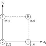
Figure 8.17 : Geometrical representation of XOR function.
It follows from Figure 8.17 where all possible inputs are depicted in the input space and labeled with the corresponding outputs that there is no straight line to separate the points corresponding to output value 1 from the points associated with output value 0. This implies that the neurons need to be connected into a network in order to solve more complicated tasks, as it is the case of the human nervous system.
The above-mentioned principles will be illustrated through an example of a neural network whose computational dynamics will be described in more detail and also its geometrical interpretation will be outlined. A fixed architecture of a multilayered neural network is considered . Further, suppose that each connection in this network is labeled with synaptic weights, i.e. a configuration of the multilayered network is given. At the beginning, the states of input layer neurons are assigned to a generally real network input and the remaining (hidden and output) neurons are passive. The computation further proceeds at discrete time steps. At time 1, the states of neurons from the first (hidden) layer are updated according to eq.7.3. This means that a neuron from this layer collects its inputs from the input neurons, computes its excitation level as a weighted sum of these inputs and its state (output) determines from the sign of this sum by applying the transfer function (hard limiter). Then at time 2, the states of neurons from the second (hidden) layer are updated again according to eq. 7.3. In this case, however, the outputs of neurons from the first layer represent the inputs for neurons in the second layer. Similarly, at time 3 the states of neurons in the third layer are updated, etc. Thus, the computation proceeds in the direction from the input layer to the output one so that at each time step all neurons from the respective layer are updated in parallel based on inputs collected from the preceding layer. Finally, the states of neurons in the output layer are determined which form the network output, and the computation of multilayered neural network terminates.
The geometrical interpretation of neuron function will be generalized for the function of three-layered neural network. Clearly, the neurons in the first (hidden) layer disjoin the network input space by corresponding hyperplanes into various halfspaces. Hence, the number of these halfspaces equals the number of neurons in the first layer. Then, the neurons in the second layer can, classify the intersections of some of these halfspaces, i.e. they can represent convex regions in the input space. This means that a neuron from the second layer is active if and only if the network input corresponds to a point in the input space that is located simultaneously in all halfspaces, which are classified by selected neurons from the first layer. Although the remaining neurons from the first layer are formally connected to this neuron in the topology of multilayered network, however, the corresponding weights are zero and hence, they do not influence the underlying neuron. In this case, the neurons in the second layer realize logical conjunction AND of relevant inputs; i.e. each of them is active if and only if all its inputs are 1. In Figure 8.18, the partition of input space into four halfspaces P1, P2, P3 , P 4 by four neurons from the first layer is depicted (compare with the example of multilayered architecture 3-4-3-2 in Figure 7.9 . Three convex regions are marked here that are the intersections of halfspaces K1=P1 ∩ P 2∩P 3 , K 2 =P 2 ∩ P 3∩P 4 , and K3=P1∩ P 4 . They correspond to three neurons from the second layer, each of them being active if and only if the network input is from the respective region.
The partition of the input space into convex regions can be exploited for the pattern recognition of more characters where each character is associated with one convex region. Sometimes the part of the input space corresponding to a particular image cannot be closed into a convex region. However, a non-convex area can be obtained by a union of convex regions, which is implemented by a neuron from the third (output) layer. This means that the output neuron is active if and only if the network input represents a point in the input space that is located in at least one of the selected convex regions, which are classified by neurons from the second layer. In this case, the neurons in the output layer realize logical disjunction (OR) of relevant inputs; i.e. each of them is active if and only if at least one of its inputs is 1. For example, in Figure 8.18 the output neuron is active if and only if the network input belongs to the region K1 or K2 (i.e. K1 U K2). It is clear that the non-convex regions can generally be classified by three-layered neural networks.
Figure 8.18 : Example of convex region separation.
In the preceding considerations the fact that the logical conjunction AND and disjunction OR, respectively, are computable by one neuron with the computational dynamics (eq. 7.3), has been exploited. In Figure 8.19, the neuron implementation of these functions is depicted. The unit weights (excluding bias) ensure the weighted sum of actual binary inputs (taken from the set {0,1}) to equal the number of 1’s in the input. The threshold (the bias with the opposite sign) n for AND and 1 for OR function causes the neuron to be active if and only if this number is at least n or 1, respectively. Of course, the neurons in the upper layers of a multilayered network may generally compute other functions than only a logical conjunction or disjunction. Therefore, the class of functions computable by multilayered neural networks is richer than it has been assumed in our example.
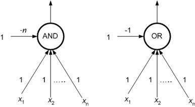
Figure 8.19 : Neuron implementation of AND and OR.
In addition, the geometrical interpretation of the multilayered neural network will be illustrated by the above-mentioned important example of logical function, the exclusive disjunction (XOR). This function is not computable by one neuron with the computational dynamics (eq.7.3).
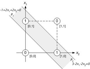
Figure 8.20 : Geometrical interpretation of XOR computation by two-layered network.
As it can be seen in Figure 8.20, the (two-dimensional) network inputs for which the output value of XOR function is 1, can be closed by the intersection of two halfspaces (half-planes) P1 , P 2 bounded by hyperplanes (straight lines), into a convex region. Therefore, the XOR function can be implemented by the two-layered neural network 2-2-1 (with one hidden layer), which is depicted in Figure 8.21 .
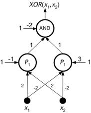
Figure 8.21 : Two layered network for XOR computation.
The equation of a line whose coordinates of two points are known is given as;
![]() (8.31)
(8.31)
Thus can be solved as;
![]() (8.32)
(8.32)
In the above example the two coordinates of the first hyperplane can be
found as ![]() and
and
![]() . Using
these values in eq.8.7 will yield;
. Using
these values in eq.8.7 will yield;
![]() (8.33)
(8.33)
which is the equation of the first hyperplane. The equation of the other hyperplane is treated similary which is
![]() (8.34)
(8.34)
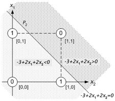
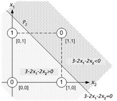
Note that any point below eq.8.31 yields the result of y=0 since
![]() (see Figure 8.22
a). To give way to the network implementation, this result should be avoided.
Thus the equation is multiplied by –1 so that any point below the
hyperplane P2 yields y=1 (see Figure 8.22 b).
(see Figure 8.22
a). To give way to the network implementation, this result should be avoided.
Thus the equation is multiplied by –1 so that any point below the
hyperplane P2 yields y=1 (see Figure 8.22 b).
(a) (b)
Figure 8.22 : The effect of the multiplication of the equation of hyperplane by –1.
Also note that the following correlations are true;
![]() Þ
Þ
![]()
![]() Þ
Þ
![]()
![]() Þ
Þ
![]()
Figure 8.23 : Block diagram of XOR gate implemented with MATLAB.
[1] Sima J. (1998). Introduction to Neural Networks, Technical Report No. V 755, Institute of Computer Science, Academy of Sciences of the Czech Republic
[2] Kröse B., and van der Smagt P. (1996). An Introduction to Neural Networks. (8th ed.) University of Amsterdam Press, University of Amsterdam.
[3] Gurney K. (1997). An Introduction to Neural Networks . (1st ed.) UCL Press, London EC4A 3DE, UK.
[4] Paplinski A.P. Neural Nets. Lecture Notes, Dept. of Computer Sciences and Software Eng., Manash Universtiy, Clayton-AUSTRALIA