Maximum-likelihood and Bayesian parameter estimation techniques assume that the forms for the underlying probability densities were known, and that we will use the training samples to estimate the values of their parameters. In this chapter, we shall instead assume we know the proper forms for the discriminant functions, and use the samples to estimate the values of parameters of the classifier. Some of the discriminant functions are statistical and some of them are not. None of them, however, requires knowledge of the forms of underlying probability distributions, and in this limited sense, they can be said to be nonparametric.
Linear discriminant functions have a variety of pleasant analytical properties. They can be optimal if the underlying distributions are cooperative, such as Gaussians having equal covariance, as might be obtained through an intelligent choice of feature detectors. Even when they are not optimal, we might be willing to sacrifice some performance in order to gain the advantage of their simplicity. Linear discriminant functions are relatively easy to compute and in the absence of information suggesting otherwise, linear classifiers are attractive candidates for initial, trial classifiers.
The problem of finding a linear discriminant function will be formulated as a problem of minimizing a criterion function. The obvious criterion function for classification purposes is the sample risk , or training error - the average loss incurred in classifying the set of training samples. It is difficult to derive the minimum-risk linear discriminant, and for that reason it will be suitable to investigate several related criterion functions that are analytically more tractable. Much of our attention will be devoted to studying the convergence properties and computational complexities of various gradient descent procedures for minimizing criterion functions. The similarities between many of the procedures sometimes make it difficult to keep the differences between them clear.
A discriminant function that is a linear combination of the components of x can be written as
![]() (9.1)
(9.1)
where w is the weight vector and w 0 the bias or threshold weight. Linear discriminant functions are going to be studied for the two-category case, multi-category case, and general case (Figure 9.1). For the general case there will be c such discriminant functions, one for each of c categories.
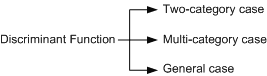
Figure 9.1: Linear discriminant functions.
For a discriminant function of the form of eq.9.1, a two-category classifier implements the following decision rule: Decide w 1 if g(x)>0 and w 2 if g(x)< 0. Thus, x is assigned to w 1 if the inner product w T x exceeds the threshold – w 0 and to w 2 otherwise. If g(x)= 0, x can ordinarily be assigned to either class, or can be left undefined. The equation g(x) = 0 defines the decision surface that separates points assigned to w 1 from points assigned to w 2. When g(x) is linear, this decision surface is a hyperplane. If x 1 and x 2 are both on the decision surface, then
![]() (9.2)
(9.2)
or
![]() (9.3)
(9.3)
and this shows that w is normal to any vector lying in the hyperplane. In general, the hyperplane H divides the feature space into two half-spaces: decision region R 1 for w1 and region R 2 for w2 . Because g(x)> 0 if x is in R 1 , it follows that the normal vector w points into R 1 . It is sometimes said that any x in R 1 is on the positive side of H, and any x in R 2 is on the negative side (Figure 9.2).
The discriminant function g(x) gives an algebraic measure of the distance from x to the hyperplane. The easiest way to see this is to express x as
![]() (9.4)
(9.4)
where xp is the normal projection of x onto H, and r is the desired algebraic distance which is positive if x is on the positive side and negative if x is on the negative side. Then, because g(xp) = 0,
![]()
![]()
![]()
![]() Since
Since
![]() then
then
![]()
![]()
![]() (9.5)
(9.5)
or
![]() (9.6)
(9.6)
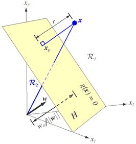
Figure 9.2: The linear decision boundary H separates the feature space into two half-spaces.
In particular,
the distance from the origin to H is given by
![]() . If w
0
>
0, the origin is on
the positive side of H, and if w
0
<0, it is on the
negative side. If w
0=
0, then g(x)
has the homogeneous form
. If w
0
>
0, the origin is on
the positive side of H, and if w
0
<0, it is on the
negative side. If w
0=
0, then g(x)
has the homogeneous form
![]() , and the hyperplane passes through the
origin (Figure 9.2). A linear discriminant function divides the feature space
by a hyperplane decision surface. The orientation of the surface is determined
by the normal vector w, and the location of the surface is
determined by the bias
w
0
.
The discrim
inant function g(x)
is proportional to the signed distance from x to the hyperplane, with g(x)>0
when x is on
the
positive side, and g(x)<0 when x is on the
negative side.
, and the hyperplane passes through the
origin (Figure 9.2). A linear discriminant function divides the feature space
by a hyperplane decision surface. The orientation of the surface is determined
by the normal vector w, and the location of the surface is
determined by the bias
w
0
.
The discrim
inant function g(x)
is proportional to the signed distance from x to the hyperplane, with g(x)>0
when x is on
the
positive side, and g(x)<0 when x is on the
negative side.
There is more than one way to devise multicategory classifiers employing linear discriminant functions. For example, we might reduce the problem to c two-class problems, where the ith problem is solved by a linear discriminant function that separates points assigned to wi, from those not assigned to w 1 . A more extravagant approach would be to use c( c- 1)/2 linear discriminants, one for every pair of classes. As illustrated in Figure 9.3 , both of these approaches can lead to regions in which the classification is undefined. We shall avoid this problem by defining c linear discriminant functions
![]() (9.7)
(9.7)
and assigning x
to wi if
![]() for all
j
¹
i;
in case of ties, the classification is
left undefined. The resulting classifier is called a
linear machine.
A linear machine divides the feature space into c decision
regions (Figure 9.4), with gj(x) being the largest discriminant
if x is in region
Ri
. If
R
i
and
R
j
are
contiguous, the boundary between them is a portion of the hyperplane
H
ij
defined by
for all
j
¹
i;
in case of ties, the classification is
left undefined. The resulting classifier is called a
linear machine.
A linear machine divides the feature space into c decision
regions (Figure 9.4), with gj(x) being the largest discriminant
if x is in region
Ri
. If
R
i
and
R
j
are
contiguous, the boundary between them is a portion of the hyperplane
H
ij
defined by
![]() or
or
![]()
It follows at once that
![]() is normal to Hij and
the signed distance from x to Hij is given by
is normal to Hij and
the signed distance from x to Hij is given by

Thus, with the linear machine it is not the weight vectors themselves but their differences that are important. While there are c(c-1)/2 pairs of regions, they need not all be contiguous, and the total number of hyperplane segments appearing in the decision surfaces is often fewer than c(c-1)/2, as shown in Figure 9.4.
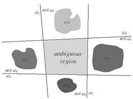
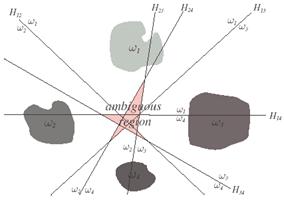
Figure 9.3: Linear decision boundaries for a four-class problem with undefined regions.
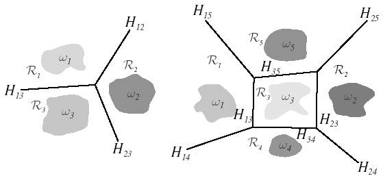
Figure 9.4: Decision boundaries defined by a linear machine.
The linear discriminant function g(x) can be written as
![]() (9.8)
(9.8)
where the coefficients wi are the components of the weight vector w. By adding additional terms involving the products of pairs of components of x, we obtain the quadratic discriminant function
![]() (9.9)
(9.9)
Because xixj= xjxi we can assume that wij=wji with no loss in generality. The eq.9.9 evaluates in 2D feature space as
![]()
![]()
![]() (9.10)
(9.10)
where eq.9.9 and 9.10 are equivalent. Thus, the quadratic discriminant function has an additional d(d+l)/2 coefficients at its disposal with which to produce more complicated separating surfaces. The separating surface defined by g(x)=0 is a second-degree or hyperquadric surface. If the symmetric matrix W=[wij], where the elements wij are the weights of the last term in eq.9.9, is nonsingular the linear terms in g(x) can be eliminated by translating the axes. The basic character of the separating surface can be described in terms of the scaled matrix
![]() where
where
![]() and W=[wij].
and W=[wij].
Types of Quadratic Surfaces:
The types of quadratic separating surfaces that arise in the general multivariate Gaussian case are as follows.
1.
If ![]() is
a positive multiple of the identity matrix, the separating surface is a hypersphere
such that:
is
a positive multiple of the identity matrix, the separating surface is a hypersphere
such that: ![]() ,
where k
³
0. Also note that, hypersphere is defined as
,
where k
³
0. Also note that, hypersphere is defined as
![]()
2.
If ![]() is
positive definite, the separating surfaces is a hyperellipsoid whose
axes are in the directions of the eigenvectors of
is
positive definite, the separating surfaces is a hyperellipsoid whose
axes are in the directions of the eigenvectors of
![]() .
.
3.
If none of the above cases holds, that is, some of the eigenvalues
of ![]() are
positive and others are negative, the surface is one of the varieties of types
of hyperhyperboloids.
are
positive and others are negative, the surface is one of the varieties of types
of hyperhyperboloids.
By continuing to add terms such as wijkxixjxk, we can obtain the class of polynomial discriminant functions. These can be thought of as truncated series expansions of some arbitrary g(x), and this in turn suggest the generalized linear discriminant function
![]() (9.11)
(9.11)
or
![]() (9.12)
(9.12)
where a
is now a ![]() -dimensional
weight vector and where the
-dimensional
weight vector and where the
![]() functions yi(x)
can be arbitrary functions of x. Such functions might be computed by a
feature detecting subsystem. By selecting these functions judiciously and
letting
functions yi(x)
can be arbitrary functions of x. Such functions might be computed by a
feature detecting subsystem. By selecting these functions judiciously and
letting ![]() be
sufficiently large, one can approximate any desired discriminant function by
such an expansion. The resulting discriminant function is not linear in x, but
it is linear in y. The
be
sufficiently large, one can approximate any desired discriminant function by
such an expansion. The resulting discriminant function is not linear in x, but
it is linear in y. The
![]() functions yi(x)
merely map points in d-dimensional x-space to points in
functions yi(x)
merely map points in d-dimensional x-space to points in
![]() -dimensional y-space.
The homogeneous discriminant
-dimensional y-space.
The homogeneous discriminant
![]() separates points in this transformed
space by a hyperplane passing through the origin. Thus, the mapping from x
to y reduces the problem to one of finding a homogeneous linear
discriminant function.
separates points in this transformed
space by a hyperplane passing through the origin. Thus, the mapping from x
to y reduces the problem to one of finding a homogeneous linear
discriminant function.
Some of the advantages and disadvantages of this approach can be clarified by considering a simple example. Let the quadratic discriminant function be
g(x)=a 1 + a 2 x+ a3 x 2 (9.13)
so that the three-dimensional vector y is given by
 (9.14)
The mapping from x to y is illustrated in Figure 9.5. The data remain inherently one-dimensional, because varying x causes y to trace out a curve in three dimensions
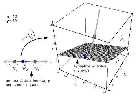
Figure 9.5: The mapping y= (1 x x2)T takes a line and transforms it to a parabola.
The mapping from x to y is illustrated in Figure 9.5. The data remain inherently one-dimensional, because varying x causes y to trace out a curve in three dimensions.
The plane
![]() defined by
defined by
![]() =0 divides the y-space
into two decision regions
=0 divides the y-space
into two decision regions
![]() and
and
![]() . Figure 5.6 shows the
separating plane corresponding to a=(-1, 1, 2)
T
, the
decision regions
. Figure 5.6 shows the
separating plane corresponding to a=(-1, 1, 2)
T
, the
decision regions ![]() and
and
![]() , and their
corresponding decision regions
, and their
corresponding decision regions
![]() and
and
![]() in the original x-space. The
quadratic discriminant function g(x)=-1+x+
2x2 is positive if x
<
-1 or if x
>
0.5
. Even with relatively simple functions yi(x),
decision surfaces induced in an x-space can be fairly complex.
in the original x-space. The
quadratic discriminant function g(x)=-1+x+
2x2 is positive if x
<
-1 or if x
>
0.5
. Even with relatively simple functions yi(x),
decision surfaces induced in an x-space can be fairly complex.
While it may be hard to realize the potential benefits of a generalized linear discriminant function, we can at least exploit the convenience of being able to write g(x) in the homogeneous form aty. In the particular case of the linear discriminant function we have
![]() (9.15)
(9.15)
where we set x 0 =1. Thus we can write
 (9.16)
and y is sometimes called an augmented feature vector. Likewise, an augmented weight vector can be written as:
 (9.17)
This mapping from d-dimensional x-space to (d+1)-dimensional y-space is mathematically trivial but nonetheless quite convenient. By using this mapping we reduce the problem of finding a weight vector w and a threshold weight w 0 to the problem of finding a single weight vector a.
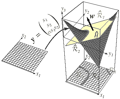
Figure 9. 6: The mapping y= (1 x x2)T takes a line and transforms it to a parabola.
Suppose now that we have a set of n samples y 1 ,…, y n , some labeled w 1 and some labeled w 2 . We want to use these samples to determine the weights a in a linear discriminant function g(x) =a T y . If there exists a solution for which the probability of error is very low, then we are going to look for a weight vector that classifies all of the samples correctly. If such a weight vector exists, the samples are said to be linearly separable.
A sample y i is classified correctly if a T y i >0 and y i is labeled w1 or if a T y i <0 and y i is labeled w2. This suggests a “normalization” that simplifies the treatment of the two-category case, namely, the replacement of all samples labeled w2 by their negatives. With the “normalization” we can forget the labels and look for a weight vector a such that a T y i >0 for all of the samples. Such a weight vector is called a separating vector or more generally a solution vector.
The weight vector a can be thought of as specifying a point in weight space. Each sample y i places a constraint on the possible location of a solution vector. The equation a T y i =0 defines a hyperplane through the origin of weight space having y i as a normal vector. The solution vector must be on the positive side of every hyperplane. Thus, a solution vector must lie in the intersection of n half-spaces; indeed any vector in this region is a solution vector. The corresponding region is called the solution region, and it should not be confused with the decision region in feature space corresponding to any particular category. A two-dimensional example illustrating the solution region for unnormalized case is shown in Figure 9.7 and for the normalized case in Figure 9.8.
From this discussion, it should be clear that the solution vector is
not unique. There are several ways to impose additional requirements to
constrain the solution vector. One possibility is to seek a unit-length weight
vector that maximizes the minimum distance from the samples to the separating
plane. Another possibility is to seek the minimum-length weight vector
satisfying a
T
y
i³b
for all i, where b is a positive constant called the
margin.
As shown in Figure 9.9, the solution region resulting form the
intersections of the half spaces for which a
T
y
i
³b
>0 lies within the previous solution region, being insulated from
the old boundaries by the distance b/
![]() .
.
The motivation behind these attempts to find a solution vector closer to the “middle” of the solution region is the natural belief that the resulting solution is more likely to classify new test samples correctly. In most of the cases, we shall be satisfied with any solution strictly within the solution region. Our chief concern will be to see that any iterative procedure used does not converge to a limit point on the boundary. This problem can always be avoided by the introduction of a margin, that is, by requiring that a T y i ³b>0 for all i.
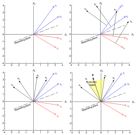
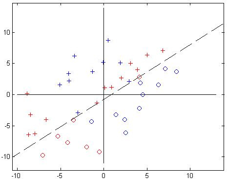
Figure 9. 7: Four training samples, blue for w1, red for w2 and the solution region in feature space. The raw data is shown. The solution vectors leads to a plane that separates the patterns from the two categories.
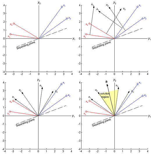
Figure 9. 8: The four training samples of Figure 9.7 and the solution region in feature space. The red points are normalized, that is, changed in sign. Now the solution vector leads to a plane that places all “normalized” points on the same side.
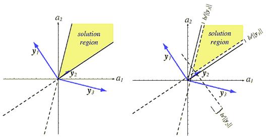
Figure 9.9: The effect of margin on the solution region.
The approach we shall take to finding a solution to the set of linear inequalities a T y i > 0 will be to define a criterion function J (a) that is minimized if a is a solution vector. This reduces our problem to one of minimizing a scalar function- a problem that can often be solved by a gradient descent procedure (Figure 9.10).
![]()
Figure 9.10: Gradient descent procedures.
Basic gradient descent is very simple. We start with some arbitrarily chosen weight vector a(1) and compute the gradient vector ÑJ (a(1)). The next value a(2) is obtained by moving some distance from a(1) in the direction of steepest descent, i.e., along the negative of the gradient. In general, a(k+1) is obtained from a(k) by the equation
![]() (9.18)
(9.18)
where h is a positive scale factor or learning rate that sets the step size. We hope that such a sequence of weight vectors will converge to a solution minimizing J(a). In algorithmic form we have:
Algorithm (Basic Gradient Descent)
begin initialize a, threshold q , h(.), k¬0
do k ¬k+1
a
¬
![]()
until ![]()
return a
end
The many problems associated with gradient descent procedures are well known. One that will confront us is the choice of the learning rate h ( k ). If h(k) is too small, convergence is needlessly slow, whereas if h(k) is too large, the correction process will overshoot and can even diverge.
We now consider a principled method for setting the learning rate. Suppose that the criterion function can be well approximated by the second-order expansion around a value a(k) as
![]() (9.19)
(9.19)
where H is the Hessian matrix of second partial derivatives ¶2 J/¶ ai ¶ j evaluated as a(k). Then, substituting a(k+1) from eq.9.18 into eq.9.19 we find
![]() (9.20)
(9.20)
From this it follows that J(a(k+1)) can be minimized by the choice
![]() (9.21)
(9.21)
where H depends on a, and thus indirectly on k. This then is the optimal choice of h (k) given the assumptions mentioned. Note that if the criterion function J(a) is quadratic through the region of interest, then H is constant and h is a constant independent of k.
An alternative approach obtained by ignoring eq.9.18 and choosing a(k+1) to minimize the second-order expansion, is Newton’s algorithm:
Algorithm (Newton Descent)
begin initialize a, threshold q
do
a
¬ a
-
![]()
until ![]()
return a
end
Newton’s algorithm works for the quadratic error functions, but not in the nonquadratic error functions of multilayer neural networks. Newton’s algorithm will usually give a greater improvement per step than simple gradient descent algorithm, even with the optimal value of h (k). However, Newton’s algorithm is not applicable if the Hessian matrix H is singular. It often takes less time to set h(k) to a constant h that is smaller than necessary and make a few more corrections than it is to compute the optimal h (k) at each step.
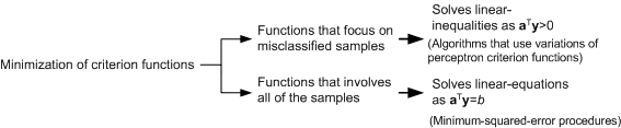
Figure 9.11: Minimizing the perceptron criterion function.
Batch Perceptron Algorithm: The Perceptron criterion function (Figure 9.11)is given by
![]() (9.22)
(9.22)
where y
(a) is
the set of samples
misclassified
by a.
(If no samples are misclassified,
y is empty and we define
Jp
to be zero.) Because
![]() £
0 if y is
misclassified.
Jp(a)
is never
negative, being zero only if a is a solution vector or if a is on the
decision boundary. Geometrically,
Jp
(a)
is proportional to the sum of the distances from the misclassified
samples to the decision boundary.
£
0 if y is
misclassified.
Jp(a)
is never
negative, being zero only if a is a solution vector or if a is on the
decision boundary. Geometrically,
Jp
(a)
is proportional to the sum of the distances from the misclassified
samples to the decision boundary.
The basic
gradient descent algorithm uses the gradient
![]() (the first derivative). From eq.9.22
the jth component of the gradient is
(the first derivative). From eq.9.22
the jth component of the gradient is
![]() (9.23)
(9.23)
Using eq. 9.23 in gradient descent algorithm, the update rule becomes
![]()
![]()
![]() (9.24)
(9.24)
where y k is the set of samples misclassified by a(k). Thus the Perceptron algorithm is as follows:
Algorithm (Batch Perceptron)
begin initialize a, h (.), criterion q , k¬0
do k ¬k+1
a
¬
![]()
until ![]()
return a
end
Thus, the batch Perceptron algorithm (Figure 9.12) for finding a solution vector can be stated very simply: The next weight vector is obtained by adding some multiple of the sum of the misclassified samples to the present weight vector. We use the term “batch” to refer to the fact that (in general) a large group of samples is used when computing each weight update.
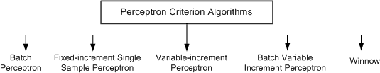
Figure 9.12: Algorithms that use perceptron criterion functions.
Fixed-increment Single Sample Perceptron Algorithm: The fixed-increment rule for generating a sequence of weight vectors can be written as
![]()
![]() (9.25)
(9.25)
where the sequence of samples using superscripts—that is, by y1, y2…. yk where each yk is one of the n samples y 1 , y 2 …. yn, and where each yk is misclassified, and a T (k)y k £ 0 for all k. If we let n denote the total number of patterns, the algorithm is as follows:
Algorithm (Fixed-Increment Single-Sample Perceptron)
begin initialize a, k ¬0
do k ¬k+1 (mod n)
if yk is misclassified by a then a ¬a +y k
until all patterns properly classified
return a
end
The fixed-increment Perceptron rule is the simplest of many algorithms for solving systems of linear inequalities. Geometrically, its interpretation in weight space is particularly clear. Because a (k) misclassifies yk, a (k) is not on the positive side of the yk hyperplane a T y k =0. The addition of yk to a (k) moves the weight vector directly toward and perhaps across this hyperplane. Whether the hyperplane is crossed or not, the new inner product, a T (k+1)yk is larger than the old inner product a T (k)yk by the amount ║ y k║2 , and the correction is hence moving the weight vector in a good direction .
Variable-increment Perceptron with Margin Algorithm: The fixed increment rule can be generalized to provide a variety of related algorithms. We shall briefly consider two variants of particular interest. The first variant introduces a variable increment h ( k ) and a margin b, and it calls for a correction whenever a T (k)yk fails to exceed the margin. The update is given by
![]()
![]() (9.26)
(9.26)
where now a T (k)yk£ b for all k. Thus for n patterns, the algorithm is:
Algorithm (Variable-Increment Perceptron with Margin)
begin initialize a, threshold q, margin b, h (.) , k ¬0
do k ¬k+1 (mod n)
if a T y k £ b then a¬ a + h(k)y k
until a T y k >b for all k
return a
end
Batch Variable-increment Perceptron Algorithm: Another variant of interest is our original gradient descent algorithm for Jp
![]()
![]() (9.27)
(9.27)
where y
k
is the set of training samples
misclassified by a(k). It is easy to see that this
algorithm will also yield a solution once one recognizes that if
![]() is a solution vector
for y
1, y2
…. yn, then it correctly classifies the
correction vector. The algorithm is as follows:
is a solution vector
for y
1, y2
…. yn, then it correctly classifies the
correction vector. The algorithm is as follows:
Algorithm (Batch Variable Increment Perceptron)
begin initialize a, h (.) , k ¬0
do k ¬k+1 (mod n)
y
k
={}
j
=0
do
j
¬j+1
If y j is misclassified then Append yj to y k
until j = n
a
¬
a
+
![]()
until y k ={}
return a
end
The benefit of batch gradient descent is that the trajectory of the weight vector is smoothed, compared to that in corresponding single-sample algorithms (e.g., variable-increment algorithm), because at each update the full set of misclassified patterns is used-the local statistical variations in the misclassified patterns tend to cancel while the large-scale trend does not. Thus, if the samples are linearly separable, all of the possible correction vectors form a linearly separable set, the sequence of weight vectors produced by the gradient descent algorithm for Jp will always converge to a solution vector.
Winnow Algorithm: A close descendant of the Perceptron algorithm is the Winnow algorithm. The key difference is that while the weight vector returned by the Perceptron algorithm has components ai (i =0,…,d), in Winnow they are scaled according to 2sinh[ai]. In one version, the balanced Winnow algorithm, there are separate “positive” and “negative” weight vectors, a+ and a-, each associated with one of the two categories to be learned. Corrections on the positive weight are made if and only if a training pattern in w 1 is misclassified; conversely, corrections on the negative weight are made if and only if a training pattern in w 2 is misclassified.
Algorithm (Balanced Winnow)
begin initialize a+ , a - , h(.) , k ¬0, a >1
if Sgn[a+ T y k - a+ T y k ]¹ zk (pattern misclassified)
then if
zk
=
+1 then
![]() for all
i
for all
i
if
zk
=
-1
then ![]() for
all
i
for
all
i
return a+, a-
end
There are two main benefits of such a version of the Winnow algorithm. The first is that during training each of the two constituent weight vectors moves in a uniform direction and this means that for separable data the “gap,” determined by these two vectors, can never increase in size. The second benefit is that convergence is generally faster than in a Perceptron, because for proper setting of learning rate, each constituent weight does not overshoot its final value. This benefit is especially pronounced whenever a large number of irrelevant or redundant features are present.
The criterion functions focus their attention on the misclassified samples. The criterion functions that are based on minimum squared-error involve all of the samples. Where previously we have sought a weight vector a making all of the inner products a T y i positive, now we shall try to make a T y i =bi, where the bi are some arbitrarily specified positive constants. Thus, we have replaced the problem of finding the solution to a set of linear inequalities with the more stringent but better understood problem of finding the solution to a set of linear equations.
The treatment
of simultaneous linear equations is simplified by introducing matrix notation.
Let Y be the n-by-
![]() matrix (
matrix (
![]() = d
+ 1) whose ith row is the vector
= d
+ 1) whose ith row is the vector
![]() , and let b
be the column vector b
=
(b
1
…
bn )T. Then our problem is to find a weight vector a satisfying
, and let b
be the column vector b
=
(b
1
…
bn )T. Then our problem is to find a weight vector a satisfying
 or
Ya=b
(9.28)
or
Ya=b
(9.28)
If Y were nonsingular, we could write a=Y-1b and obtain a formal solution at once. However, Y is rectangular, usually with more rows than columns. When there are more equations than unknowns, a is over-determined, and ordinarily no exact solution exists. However, we can seek a weight vector a that minimizes some function of the error between Ya and b. If we define the error vector e by
e =Ya- b (9. 29)
then one approach is to try to minimize the squared length of the error vector. This is equivalent to minimizing the sum-of-squared-error criterion function
![]() (9.30)
(9.30)
The problem of minimizing the sum of squared error can be solved by a gradient search procedure. A simple closed-form solution can also be found by forming the gradient
![]() (9.31)
(9.31)
and setting it equal to zero. This yields the necessary condition
![]() (9.32)
(9.32)
and in this way
we have converted the problem of solving Ya=b to that of solving
![]() . This
celebrated equation has the great advantage that the
. This
celebrated equation has the great advantage that the
![]() -by-
-by-
![]() matrix
matrix
![]() is square and
often nonsingular. If it is nonsingular, we can solve for a uniquely as
is square and
often nonsingular. If it is nonsingular, we can solve for a uniquely as
![]() (9.33)
(9.33)
where the
![]() -by-n matrix
is called the pseudoinverse of Y. Note that if Y is square
and nonsingular, the pseudoinverse coincides with the regular inverse. Note
also that Y
†
Y
=I, but YY
†
¹I
in general.
However, a minimum-squared-error (MSE) solution always exists.
-by-n matrix
is called the pseudoinverse of Y. Note that if Y is square
and nonsingular, the pseudoinverse coincides with the regular inverse. Note
also that Y
†
Y
=I, but YY
†
¹I
in general.
However, a minimum-squared-error (MSE) solution always exists.
The MSE solution depends on the margin vector b, and different choices for b give the solution different properties. If b is fixed arbitrarily, there is no reason to believe that the MSE solution yields a separating vector in the linearly separable case. However, it is reasonable to hope that by minimizing the squared-error criterion function we might obtain a useful discriminant function in both the separable and the nonseparable cases.
Another property of the MSE solution that recommends its use is that if b=1n, it approaches a minimum mean-squared-error approximation to the Bayes discriminant function
![]() (9.34)
(9.34)
This result gives considerable insight into the MSE procedure. By approximating g 0(x), the discriminant function a T y gives direct information about the posterior probabilities
![]() and
and ![]() (9.35)
(9.35)
Unfortunately, the mean-square-error criterion places emphasis on points where p(x) is larger, rather than on points near the decision surface g 0 (x)=0. Thus, the discriminant function that “best” approximates the Bayes discriminant does not necessarily minimize the probability of error. Despite this property, the MSE solution has interesting properties and has received considerable attention in the literature.
The
![]() can be minimized by
a gradient descent procedure. Such an approach has two advantages over merely
computing the pseudoinverse: (1) It avoids the problems that arise when Y
T
Y
is singular,
and (2) it avoids the need for working with large matrices. In addition, the
computation involved is effectively a feedback scheme, which automatically
copes with some of the computational problems due to round off. Because
can be minimized by
a gradient descent procedure. Such an approach has two advantages over merely
computing the pseudoinverse: (1) It avoids the problems that arise when Y
T
Y
is singular,
and (2) it avoids the need for working with large matrices. In addition, the
computation involved is effectively a feedback scheme, which automatically
copes with some of the computational problems due to round off. Because
![]() the update rule is
the update rule is
![]()
![]() (9.36)
(9.36)
While the
![]() -by-
-by-
![]() matrix Y
T
Y
is usually smaller than the
matrix Y
T
Y
is usually smaller than the
![]() -by-n
matrix Y
†
, the storage
requirements can be reduced still further by considering the samples sequentially
and using the
Widrow-Hoff or LMS rule (least-mean-squared):
-by-n
matrix Y
†
, the storage
requirements can be reduced still further by considering the samples sequentially
and using the
Widrow-Hoff or LMS rule (least-mean-squared):
![]()
![]() (9.37)
(9.37)
or in algorithm form:
Algorithm (LMS)
begin initialize a, threshold q, h(.) , k ¬0
do k¬k+1 (mod n)
a ¬a + h (k)(bk- a T y k) y k
until
![]()
return a
end
The solution need not give a separating vector, even if one exists, as shown in Figure 9.14.
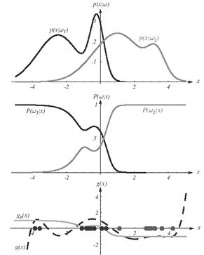
Figure 9.13: Two class-conditional densities and the posteriors. Minimizing the MSE also minimizes the mean-squared-error between a T y and the discriminant function g(x) measured over the data distribution.
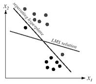
Figure 9.14: The LMS solution minimizes the sum of squares of the distances of the training points to the hyperplane and need not converge to a separating plane.
The algorithms proposed in previous sections are implemented using MATLAB. The input vectors that are used for learning are given below.
o®
![]()
+®
![]()
The point data that is used for simulation is as given below.
o
+
®
![]()
o®
![]()
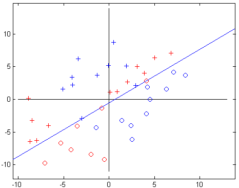
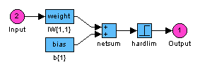
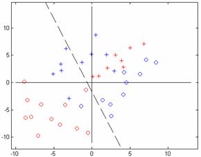
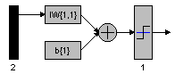
The results of the Perceptron learning rule is given for comparison. Figure 9.15 shows the network used for the perceptron-learning algorithm, the data used for learning (the blue colored plot), the classification line, and the simulation ( the red colored plot).
Algorithm: Perceptron learning rule
(a)
(b)
Figure 9. 15: Classification with perceptron learning rule algorithm. a. Learning and simulation of the given data set, b. Simulink model of the network used for the classification.
Steps required to learn the data given: 11
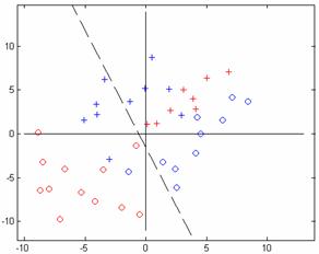
Algorithm: Batch Perceptron

(a) (b)
(c)
Figure 9.16: Batch perceptron algorithm. a. Classification after 3000 epochs, b. classification after 30000 epochs, and c. Simulink model of the network used.
Steps required to learn the data given: In actual neural-network training, often 100,000s of steps, or epochs, of the gradient-descent algorithm are required to converge to a good local minimum. (An epoch is defined to be one complete presentation of the training data.) Advanced training algorithms can reduce this large number of required epochs by several orders of magnitude. Moreover, in some of these algorithms, the learning rate will not have to be manually adjusted; rather, all necessary learning parameters are computed automatically as a function of the local second-order properties of the error surface.
Script: ccBatchPerceptron.m
Algorithm: Fixed-Increment Single Sample Perceptron
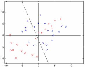
(a) (b)
(c)
Figure 9.17: Fixed-Increment Single Sample algorithm. a. Classification after 100 epochs, b. classification after 1000 epochs, and c. Simulink model of the network used.
Steps required to learn the data given: The goal cannot be achieved after 1000 epochs
Script: ccFixedIncrSingleSamplePercp.m
Algorithm: Variable-Increment Perceptron with Margin
(a)
(b)
Figure 9.18: Variable-Increment Perceptron with Margin algorithm. a. Classification after 5 epochs, b. Simulink model of the network used.
Steps required to learn the data given: 5
[1]Duda, R.O., Hart, P.E., and Stork D.G., (2001). Pattern Classification. (2nd ed.). New York: Wiley-Interscience Publication.
[2]Schalkoff R. J. (1997). Artificial Neural Networks. The McGraw-Hill Press, USA.